9 Assignment solutions
9.1 Assignment 1
We’ll use the music data set from the last session as the basis for the assignment.
Please use R to solve the tasks. When you finished the assignment, click on the “Knit to HTML” in the RStudio menu. This will create an html document in the folder in which the assignment1.Rmd file is stored. Open this file in your browser to check if everything is correct. If you are happy with the output, pleas submit the .html-file via the assignment on Learn@WU using the following file name: “assignment1_studendID_lastname.html”.
We’ll first load the data that is needed for the assignment.
library(dplyr)
library(psych)
library(ggplot2)

music_data <- read.csv2("https://raw.githubusercontent.com/WU-RDS/RMA2022/main/data/music_data_fin.csv",
    sep = ";", header = TRUE, dec = ",")
str(music_data)
## 'data.frame': 66796 obs. of 31 variables:
## $ isrc : chr "BRRGE1603547" "USUM71808193" "ES5701800181" "ITRSE2000050" ...
## $ artist_id : int 3679 5239 776407 433730 526471 1939 210184 212546 4938 119985 ...
## $ streams : num 11944813 8934097 38835 46766 2930573 ...
## $ weeks_in_charts : int 141 51 1 1 7 226 13 1 64 7 ...
## $ n_regions : int 1 21 1 1 4 8 1 1 5 1 ...
## $ danceability : num 50.9 35.3 68.3 70.4 84.2 35.2 73 55.6 71.9 34.6 ...
## $ energy : num 80.3 75.5 67.6 56.8 57.8 91.1 69.6 24.5 85 43.3 ...
## $ speechiness : num 4 73.3 14.7 26.8 13.8 7.47 35.5 3.05 3.17 6.5 ...
## $ instrumentalness : num 0.05 0 0 0.000253 0 0 0 0 0.02 0 ...
## $ liveness : num 46.3 39 7.26 8.91 22.8 9.95 32.1 9.21 11.4 10.1 ...
## $ valence : num 65.1 43.7 43.4 49.5 19 23.6 58.4 27.6 36.7 76.8 ...
## $ tempo : num 166 191.2 99 91 74.5 ...
## $ song_length : num 3.12 3.23 3.02 3.45 3.95 ...
## $ song_age : num 228.3 144.3 112.3 50.7 58.3 ...
## $ explicit : int 0 0 0 0 0 0 0 0 1 0 ...
## $ n_playlists : int 450 768 48 6 475 20591 6 105 547 688 ...
## $ sp_popularity : int 51 54 32 44 52 81 44 8 59 68 ...
## $ youtube_views : num 1.45e+08 1.32e+07 6.12e+06 0.00 0.00 ...
## $ tiktok_counts : int 9740 358700 0 13 515 67300 0 0 653 3807 ...
## $ ins_followers_artist : int 29613108 3693566 623778 81601 11962358 1169284 1948850 39381 9751080 343 ...
## $ monthly_listeners_artist : int 4133393 18367363 888273 143761 15551876 16224250 2683086 1318874 4828847 3088232 ...
## $ playlist_total_reach_artist: int 24286416 143384531 4846378 156521 90841884 80408253 7332603 24302331 8914977 8885252 ...
## $ sp_fans_artist : int 3308630 465412 23846 1294 380204 1651866 214001 10742 435457 1897685 ...
## $ shazam_counts : int 73100 588550 0 0 55482 5281161 0 0 39055 0 ...
## $ artistName : chr "Luan Santana" "Alessia Cara" "Ana Guerra" "Claver Gold feat. Murubutu" ...
## $ trackName : chr "Eu, Você, O Mar e Ela" "Growing Pains" "El Remedio" "Ulisse" ...
## $ release_date : chr "2016-06-20" "2018-06-14" "2018-04-26" "2020-03-31" ...
## $ genre : chr "other" "Pop" "Pop" "HipHop/Rap" ...
## $ label : chr "Independent" "Universal Music" "Universal Music" "Independent" ...
## $ top10 : int 1 0 0 0 0 1 0 0 0 0 ...
## $ expert_rating : chr "excellent" "good" "good" "poor" ...head(music_data)You should then convert the variables to the correct types:
music_data <-  music_data %>%
  mutate(label = as.factor(label), # convert label and genre variables to factor with values as labels
         genre = as.factor(genre)) %>% as.data.frame()
9.1.1 Q1
Create a new data frame containing the most successful songs of the artist “Billie Eilish” by filtering the original data set by the artist “Billie Eilish” and order the observations in an descending order.
billie_eilish <- music_data %>%
  select(artistName,trackName,streams) %>% #select relevant variables
  filter(artistName == "Billie Eilish") %>% #filter by artist name
  arrange(desc(streams)) #arrange by number of streams (in descending order)
billie_eilish #print output
9.1.2 Q2
Create a new data frame containing the 100 overall most successful songs in the data frame and order them descending by the number of streams.
Here you could simply arrange the whole data set by streams and then take 100 first rows using the head()-function:
top_100 <- music_data %>%
  select(artistName,trackName,streams) %>% #select relevant variables
  arrange(desc(streams)) %>% #arrange by number of streams (in descending order)
  head(100) #select first 100 observations
top_100
9.1.3 Q3
Which genres are most popular? Group the data by genre and compute the sum of streams by genre.
Using dplyr functions, you could first group the observations by genre, then summarize the streams using sum():
genres_popularity <- music_data %>%
  group_by(genre) %>% #group by genre
  summarize(streams = sum(streams)) #compute sum of streams per genre
genres_popularity
9.1.4 Q4
Which music label is most successful? Group the data by music label and compute the sum of streams by label and the average number of streams for all songs associated with a label.
Just like in the previous task, it would be enough to group the observations (in this case, by labels), and get the sums and averages of streams:
label_success <- music_data %>%
  group_by(label) %>% #group by label
  summarize(sum_streams = sum(streams),
            avg_streams = mean(streams)) #compute sum of streams and average streams per label
label_success
9.1.5 Q5
How do the songs differ in terms of the song features? Please first select the relevant variables (7 song features) and compute the descriptive statistics for these variables by genre.
All audio features (danceability, energy, speechiness, instrumentalness, liveness, valence, and tempo) are variables measured on a ratio scale, which means that we can evaluate their average values. We can use describeBy() function, which displays mean by default alongside with range and other values:
library(psych)
describeBy(select(music_data, danceability, energy,
    speechiness, instrumentalness, liveness, valence,
    tempo), music_data$genre, skew = FALSE)
##
## Descriptive statistics by group
## group: Classics/Jazz
## vars n mean sd min max range se
## danceability 1 80 46.00 18.34 7.33 83.70 76.37 2.05
## energy 2 80 30.85 19.51 0.26 85.00 84.74 2.18
## speechiness 3 80 6.11 6.55 2.46 46.70 44.24 0.73
## instrumentalness 4 80 11.34 25.65 0.00 96.10 96.10 2.87
## liveness 5 80 13.44 7.63 4.61 39.50 34.89 0.85
## valence 6 80 38.24 24.30 3.60 90.00 86.40 2.72
## tempo 7 80 113.23 33.74 56.72 232.69 175.97 3.77
## ------------------------------------------------------------
## group: Country
## vars n mean sd min max range se
## danceability 1 504 59.67 11.98 19.20 92.20 73.00 0.53
## energy 2 504 69.71 18.71 4.84 97.70 92.86 0.83
## speechiness 3 504 5.16 4.10 2.48 35.10 32.62 0.18
## instrumentalness 4 504 0.24 4.04 0.00 89.10 89.10 0.18
## liveness 5 504 23.70 21.43 3.35 98.50 95.15 0.95
## valence 6 504 58.90 21.08 7.40 96.70 89.30 0.94
## tempo 7 504 124.52 31.19 48.72 203.93 155.21 1.39
## ------------------------------------------------------------
## group: Electro/Dance
## vars n mean sd min max range se
## danceability 1 2703 66.55 11.87 22.40 97.3 74.90 0.23
## energy 2 2703 74.51 13.99 2.62 99.9 97.28 0.27
## speechiness 3 2703 7.82 6.33 2.37 47.4 45.03 0.12
## instrumentalness 4 2703 5.05 16.75 0.00 98.5 98.50 0.32
## liveness 5 2703 18.57 14.12 2.21 96.5 94.29 0.27
## valence 6 2703 47.50 21.49 3.15 97.8 94.65 0.41
## tempo 7 2703 120.74 19.42 73.99 215.9 141.91 0.37
## ------------------------------------------------------------
## group: German Folk
## vars n mean sd min max range se
## danceability 1 539 63.03 15.36 20.60 96.40 75.80 0.66
## energy 2 539 61.73 22.56 5.48 99.90 94.42 0.97
## speechiness 3 539 9.80 10.20 2.45 49.90 47.45 0.44
## instrumentalness 4 539 1.75 10.02 0.00 96.10 96.10 0.43
## liveness 5 539 18.65 15.38 1.91 98.80 96.89 0.66
## valence 6 539 56.07 24.07 6.92 98.00 91.08 1.04
## tempo 7 539 119.38 28.53 58.69 202.12 143.43 1.23
## ------------------------------------------------------------
## group: HipHop/Rap
## vars n mean sd min max range se
## danceability 1 21131 73.05 12.30 8.39 98.00 89.61 0.08
## energy 2 21131 65.10 13.28 0.54 99.00 98.46 0.09
## speechiness 3 21131 20.92 13.55 2.54 96.60 94.06 0.09
## instrumentalness 4 21131 0.61 5.03 0.00 97.80 97.80 0.03
## liveness 5 21131 16.90 12.49 1.19 97.60 96.41 0.09
## valence 6 21131 49.04 20.73 3.33 97.90 94.57 0.14
## tempo 7 21131 121.68 28.22 38.80 230.27 191.47 0.19
## ------------------------------------------------------------
## group: other
## vars n mean sd min max range se
## danceability 1 5228 64.53 15.39 7.83 96.70 88.87 0.21
## energy 2 5228 63.91 20.46 3.32 98.80 95.48 0.28
## speechiness 3 5228 9.30 10.38 2.36 95.50 93.14 0.14
## instrumentalness 4 5228 0.72 6.32 0.00 97.00 97.00 0.09
## liveness 5 5228 21.91 20.27 1.51 99.10 97.59 0.28
## valence 6 5228 60.16 22.73 3.84 99.00 95.16 0.31
## tempo 7 5228 123.65 31.98 46.72 210.16 163.44 0.44
## ------------------------------------------------------------
## group: Pop
## vars n mean sd min max range se
## danceability 1 30069 63.74 14.46 0 98.3 98.3 0.08
## energy 2 30069 62.91 18.62 0 100.0 100.0 0.11
## speechiness 3 30069 9.85 10.20 0 95.6 95.6 0.06
## instrumentalness 4 30069 1.16 7.76 0 98.7 98.7 0.04
## liveness 5 30069 17.26 13.16 0 98.9 98.9 0.08
## valence 6 30069 50.33 22.57 0 98.7 98.7 0.13
## tempo 7 30069 120.94 28.44 0 217.4 217.4 0.16
## ------------------------------------------------------------
## group: R&B
## vars n mean sd min max range se
## danceability 1 1881 67.97 13.43 8.66 97.00 88.34 0.31
## energy 2 1881 61.25 15.80 2.46 96.10 93.64 0.36
## speechiness 3 1881 12.34 10.10 2.29 85.60 83.31 0.23
## instrumentalness 4 1881 0.96 6.86 0.00 94.20 94.20 0.16
## liveness 5 1881 16.04 11.62 2.07 89.10 87.03 0.27
## valence 6 1881 52.83 23.01 3.21 98.20 94.99 0.53
## tempo 7 1881 120.17 32.02 58.39 215.93 157.54 0.74
## ------------------------------------------------------------
## group: Reggae
## vars n mean sd min max range se
## danceability 1 121 75.06 9.33 40.40 94.40 54.00 0.85
## energy 2 121 67.61 14.91 14.50 91.10 76.60 1.36
## speechiness 3 121 11.96 8.69 2.62 36.30 33.68 0.79
## instrumentalness 4 121 1.82 9.52 0.00 86.10 86.10 0.87
## liveness 5 121 18.02 14.89 1.38 78.40 77.02 1.35
## valence 6 121 69.73 18.38 13.80 96.60 82.80 1.67
## tempo 7 121 111.80 31.03 66.86 214.02 147.17 2.82
## ------------------------------------------------------------
## group: Rock
## vars n mean sd min max range se
## danceability 1 4214 54.75 13.98 6.28 98.00 91.72 0.22
## energy 2 4214 67.77 21.37 1.37 99.80 98.43 0.33
## speechiness 3 4214 6.19 5.22 2.22 54.60 52.38 0.08
## instrumentalness 4 4214 5.69 17.47 0.00 98.20 98.20 0.27
## liveness 5 4214 18.65 14.52 2.08 98.80 96.72 0.22
## valence 6 4214 45.65 22.53 2.62 97.30 94.68 0.35
## tempo 7 4214 122.25 28.70 46.22 209.79 163.57 0.44
## ------------------------------------------------------------
## group: Soundtrack
## vars n mean sd min max range se
## danceability 1 326 52.82 16.25 15.00 91.50 76.50 0.90
## energy 2 326 52.05 21.96 1.26 97.90 96.64 1.22
## speechiness 3 326 6.82 7.51 2.42 81.80 79.38 0.42
## instrumentalness 4 326 5.02 19.37 0.00 93.50 93.50 1.07
## liveness 5 326 17.49 14.80 2.37 84.20 81.83 0.82
## valence 6 326 37.99 22.44 3.09 96.50 93.41 1.24
## tempo 7 326 119.50 30.80 60.81 205.54 144.73 1.719.1.6 Q6
How many songs in the data set are associated with each label?
You could use table() to get the number of songs by label:
table(music_data$label)##
## Independent Sony Music Universal Music Warner Music
## 22570 12390 21632 102049.1.7 Q7
Which share of streams do the different genres account for?
genre_streams <- music_data %>%
    group_by(genre) %>%
    summarise(genre_streams = sum(streams))  #first compute sum of streams by genre
genre_streams_share <- genre_streams %>%
    mutate(genre_share = genre_streams/sum(genre_streams))  #then divide the sum by the total streams
genre_streams_share
9.1.8 Q8
Create a histogram for the variable “Valence”
This is a simple plot of valence distribution across all songs in your data (we can see that it follows normal distribution):
ggplot(music_data, aes(x = valence)) + geom_histogram(binwidth = 4,
    col = "white", fill = "lavenderblush3") + labs(x = "Valence",
    y = "Frequency") + theme_minimal()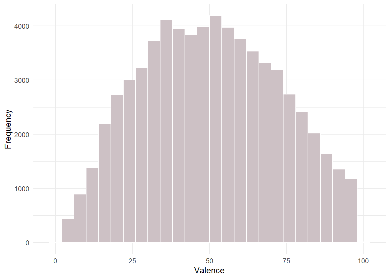
(#fig:question_8)Distribution of valence
9.1.9 Q9
Create a grouped boxplot for the variable “energy” by genre.
ggplot(music_data, aes(x = genre, y = energy, color = genre)) +
    geom_boxplot(coef = 3) + labs(x = "Genre", y = "Energy") +
    theme_minimal() + coord_flip()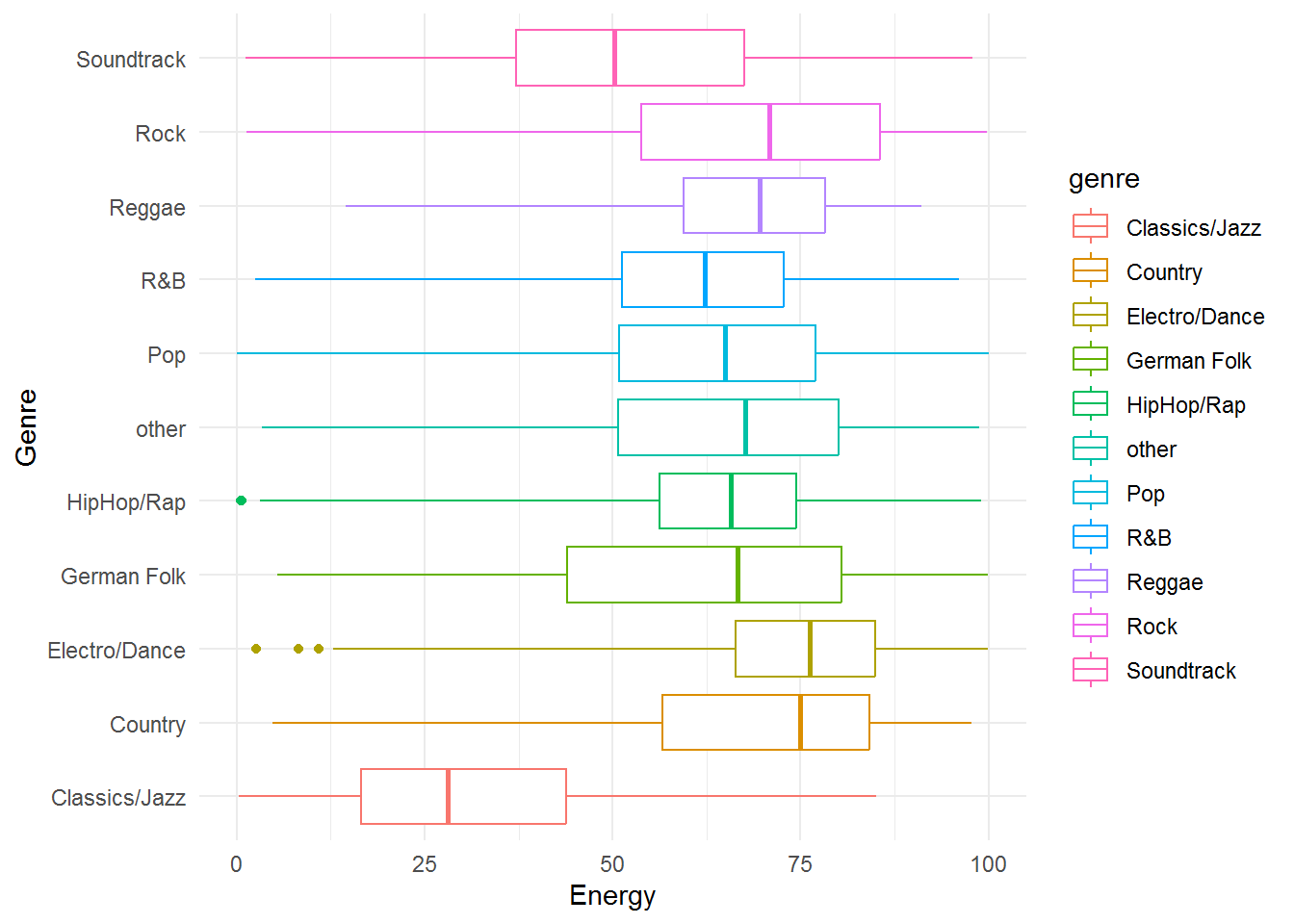
(#fig:question_9)Boxplot of energy by genre
9.1.10 Q10
Create a scatterplot for the variables “valence” and “energy”
Finally, we can visualize the relationship between valence and energy of songs in our data:
ggplot(music_data, aes(x = valence, y = energy)) +
    geom_point(shape = 1) + labs(x = "Valence", y = "Energy") +
    theme_minimal()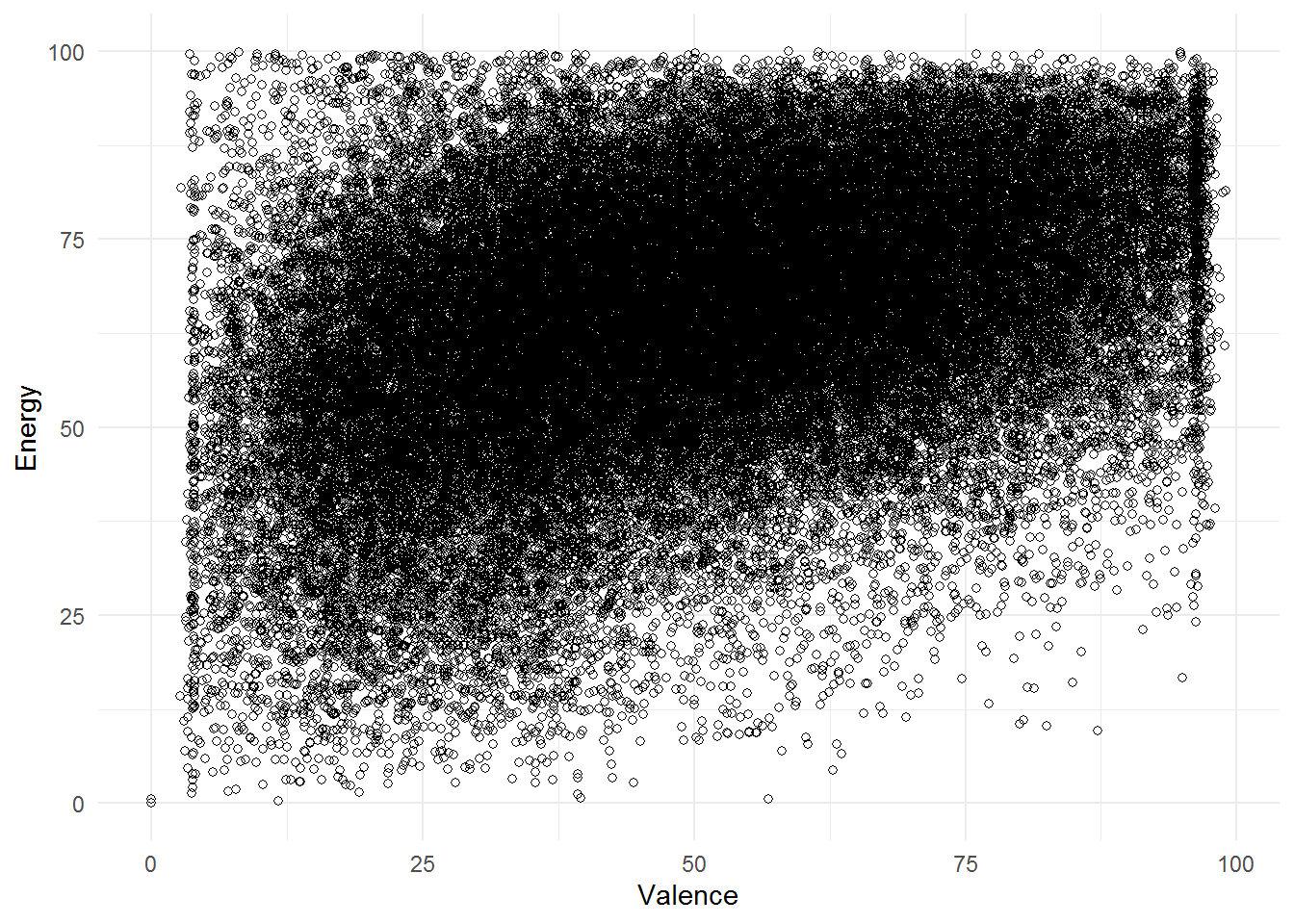
(#fig:question_10)Scatterplot of energy and valence
9.2 Assignment 2
As a marketing manager of a consumer electronics company, you are assigned the task to analyze the relative influence of different marketing activities. Specifically, you are supposed to analyze the effects of (1) TV advertising, (2) online advertising, and (3) radio advertising on the sales of fitness trackers (wristbands). Your data set consists of sales of the product in different markets (each line represents one market) from the past year, along with the advertising budgets for the product in each of those markets for three different media: TV, online, and radio.
The following variables are available to you:
- Sales (in thousands of units)
- TV advertising budget (in thousands of Euros)
- Online advertising budget (in thousands of Euros)
- Radio advertising budget (in thousands of Euros)
Please conduct the following analyses:
- Formally state the regression equation, which you will use to determine the relative influence of the marketing activities on sales.
- Describe the model variables using appropriate statistics and plots
- Estimate a multiple linear regression model and interpret the model results:
- Which variables have a significant influence on sales and what is the interpretation of the coefficients?
- How do you judge the fit of the model? Please also visualize the model fit using an appropriate graph.
- What sales quantity would you predict based on your model for a product when the marketing activities are planned as follows: TV: EUR 150 thsd., Online: EUR 26 thsd., Radio: EUR 15 thsd.? Please provide the equation you used for your prediction.
When you are done with your analysis, click on “Knit to HTML” button above the code editor. This will create a HTML document of your results in the folder where the “assignment2.Rmd” file is stored. Open this file in your Internet browser to see if the output is correct. If the output is correct, submit the HTML file via Learn@WU. The file name should be “assignment2_studendID_name.html”.
library(tidyverse)
library(psych)
library(Hmisc)
library(ggstatsplot)
options(scipen = 999)

sales_data <- read.table("https://raw.githubusercontent.com/IMSMWU/MRDA2018/master/data/assignment4.dat",
    sep = "\t", header = TRUE)  #read in data
sales_data$market_id <- 1:nrow(sales_data)
head(sales_data)str(sales_data)## 'data.frame': 236 obs. of 5 variables:
## $ tv_adspend : num 68.6 136.6 14.5 214.6 285 ...
## $ online_adspend: num 10.3 29 44.3 26.2 13.9 74.9 31.1 14.1 24.5 13.9 ...
## $ radio_adspend : int 24 40 25 40 31 24 12 9 38 18 ...
## $ sales : num 8.6 15.8 11.8 17.1 17.4 24.4 19.5 4.7 20.7 19.5 ...
## $ market_id : int 1 2 3 4 5 6 7 8 9 10 ...9.2.1 Q1
In a first step, we specify the regression equation. In this case, sales is the dependent variable which is regressed on the different types of advertising expenditures that represent the independent variables for product i. Thus, the regression equation is:
\[sales_{i}=\beta_0 + \beta_1 * tv\_adspend_{i} + \beta_2 * online\_adspend_{i} + \beta_3 * radio\_adspend_{i} + \epsilon\]
This equation will be used later to turn the output of the regression analysis (namely the coefficients: \(\beta_0\) - intersect coefficient, and \(\beta_1\), \(\beta_2\), and \(\beta_3\) that represent the unknown relationship between sales and advertising expenditures on TV, online channels and radio, respectively) to the “managerial” form and draw marketing conclusions.
9.2.2 Q2
The descriptive statistics for the variables can be checked using the describe() function:
psych::describe(sales_data)## vars n mean sd median trimmed mad min max range skew
## tv_adspend 1 236 148.65 89.77 141.85 147.45 117.27 1.1 299.6 298.5 0.12
## online_adspend 2 236 25.61 14.33 24.35 24.70 14.53 1.6 74.9 73.3 0.61
## radio_adspend 3 236 27.70 12.57 27.00 27.36 13.34 2.0 63.0 61.0 0.22
## sales 4 236 14.83 5.40 14.15 14.72 5.93 1.4 29.0 27.6 0.16
## market_id 5 236 118.50 68.27 118.50 118.50 87.47 1.0 236.0 235.0 0.00
## kurtosis se
## tv_adspend -1.26 5.84
## online_adspend 0.08 0.93
## radio_adspend -0.53 0.82
## sales -0.57 0.35
## market_id -1.22 4.44Inspecting the correlation matrix reveals that the sales variable is positively correlated with TV advertising and online advertising expenditures. The correlations among the independent variables appear to be low to moderate.
rcorr(as.matrix(sales_data[, c("sales", "tv_adspend",
    "online_adspend", "radio_adspend")]))
## sales tv_adspend online_adspend radio_adspend
## sales 1.00 0.78 0.54 -0.04
## tv_adspend 0.78 1.00 0.05 0.03
## online_adspend 0.54 0.05 1.00 -0.07
## radio_adspend -0.04 0.03 -0.07 1.00
##
## n= 236
##
##
## P
## sales tv_adspend online_adspend radio_adspend
## sales 0.0000 0.0000 0.5316
## tv_adspend 0.0000 0.4127 0.6735
## online_adspend 0.0000 0.4127 0.2790
## radio_adspend 0.5316 0.6735 0.2790Since we have continuous variables, we use scatterplots to investigate the relationship between sales and each of the predictor variables.
ggplot(sales_data, aes(x = tv_adspend, y = sales)) +
    geom_point(shape = 1) + geom_smooth(method = "lm",
    fill = "gray", color = "lavenderblush3", alpha = 0.1) +
    theme_minimal()
ggplot(sales_data, aes(x = online_adspend, y = sales)) +
    geom_point(shape = 1) + geom_smooth(method = "lm",
    fill = "gray", color = "lavenderblush3", alpha = 0.1) +
    theme_minimal()
ggplot(sales_data, aes(x = radio_adspend, y = sales)) +
    geom_point(shape = 1) + geom_smooth(method = "lm",
    fill = "gray", color = "lavenderblush3", alpha = 0.1) +
    theme_minimal()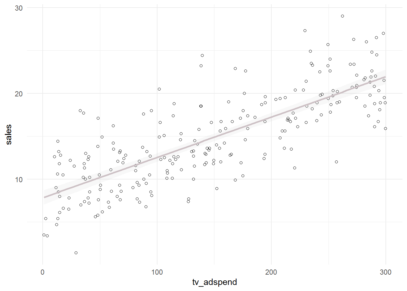
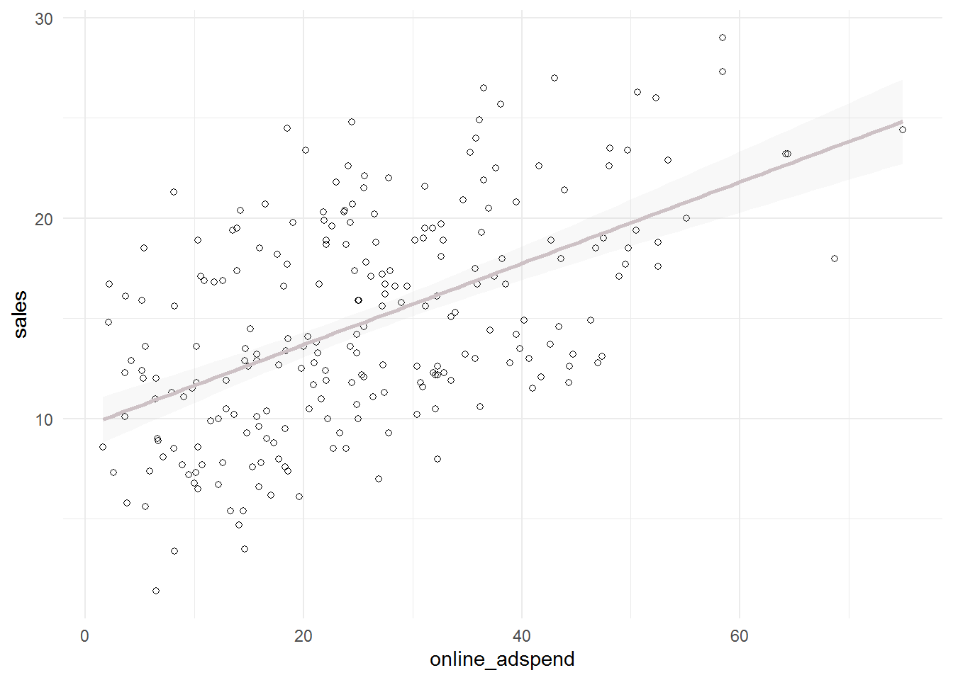
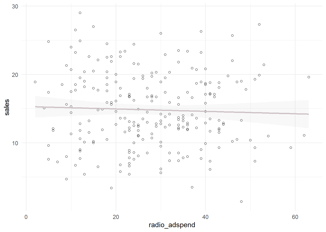
The plots including the fitted lines from a simple linear model already suggest that there might be a positive linear relationship between sales and TV- and online-advertising. However, there does not appear to be a strong relationship between sales and radio advertising.
Further steps include estimate of a multiple linear regression model in order to determine the relative influence of each type of advertising on sales.
9.2.3 Q3
The estimate the model, we will use the lm() function:
linear_model <- lm(sales ~ tv_adspend + online_adspend +
    radio_adspend, data = sales_data)
In a next step, we will investigate the results from the model using the summary() function.
summary(linear_model)##
## Call:
## lm(formula = sales ~ tv_adspend + online_adspend + radio_adspend,
## data = sales_data)
##
## Residuals:
## Min 1Q Median 3Q Max
## -5.1113 -1.4161 -0.0656 1.3233 5.5198
##
## Coefficients:
## Estimate Std. Error t value Pr(>|t|)
## (Intercept) 3.604140 0.460057 7.834 0.000000000000169 ***
## tv_adspend 0.045480 0.001491 30.508 < 0.0000000000000002 ***
## online_adspend 0.186859 0.009359 19.965 < 0.0000000000000002 ***
## radio_adspend -0.011469 0.010656 -1.076 0.283
## ---
## Signif. codes: 0 '***' 0.001 '**' 0.01 '*' 0.05 '.' 0.1 ' ' 1
##
## Residual standard error: 2.048 on 232 degrees of freedom
## Multiple R-squared: 0.8582, Adjusted R-squared: 0.8564
## F-statistic: 468.1 on 3 and 232 DF, p-value: < 0.00000000000000022For each of the individual predictors, we test the following hypothesis:
\[H_0: \beta_k=0\] \[H_1: \beta_k\ne0\]
where k denotes the number of the regression coefficient. In the present example, we reject the null hypothesis for tv_adspend and online_adspend, where we observe a significant effect (i.e., p-value < 0.05). However, we fail to reject the null for the “radio_adspend” variable (i.e., the effect is insignificant).
The interpretation of the coefficients is as follows:
- tv_adspend (β1): when TV advertising expenditures increase by 1000 Euro, sales will increase by 45 units;
- online_adspend (β2): when online advertising expenditures increase by 1000 Euro, sales will increase by 187 units;
- radio_adspend (β3): when radio advertising expenditures increase by 1000 Euro, sales will increase by -11 units (i.e., decrease by 11 units).
You should always provide a measure of uncertainty that is associated with the estimates. You could compute the confidence intervals around the coefficients using the confint() function.
confint(linear_model)## 2.5 % 97.5 %
## (Intercept) 2.69771633 4.51056393
## tv_adspend 0.04254244 0.04841668
## online_adspend 0.16841843 0.20529924
## radio_adspend -0.03246402 0.00952540The results show that, for example, the 95% confidence interval associated with coefficient capturing the effect of online advertising on sales is between 0.168 and 0.205.
Regarding the model fit, the R2 statistic tells us that approximately 86% of the variance can be explained by the model. This can be visualized as follows:
sales_data$yhat <- predict(linear_model)
ggplot(sales_data, aes(yhat, sales)) + geom_point(size = 2,
    shape = 1) + scale_x_continuous(name = "predicted values") +
    scale_y_continuous(name = "observed values") +
    geom_abline(intercept = 0, slope = 1) + theme_minimal()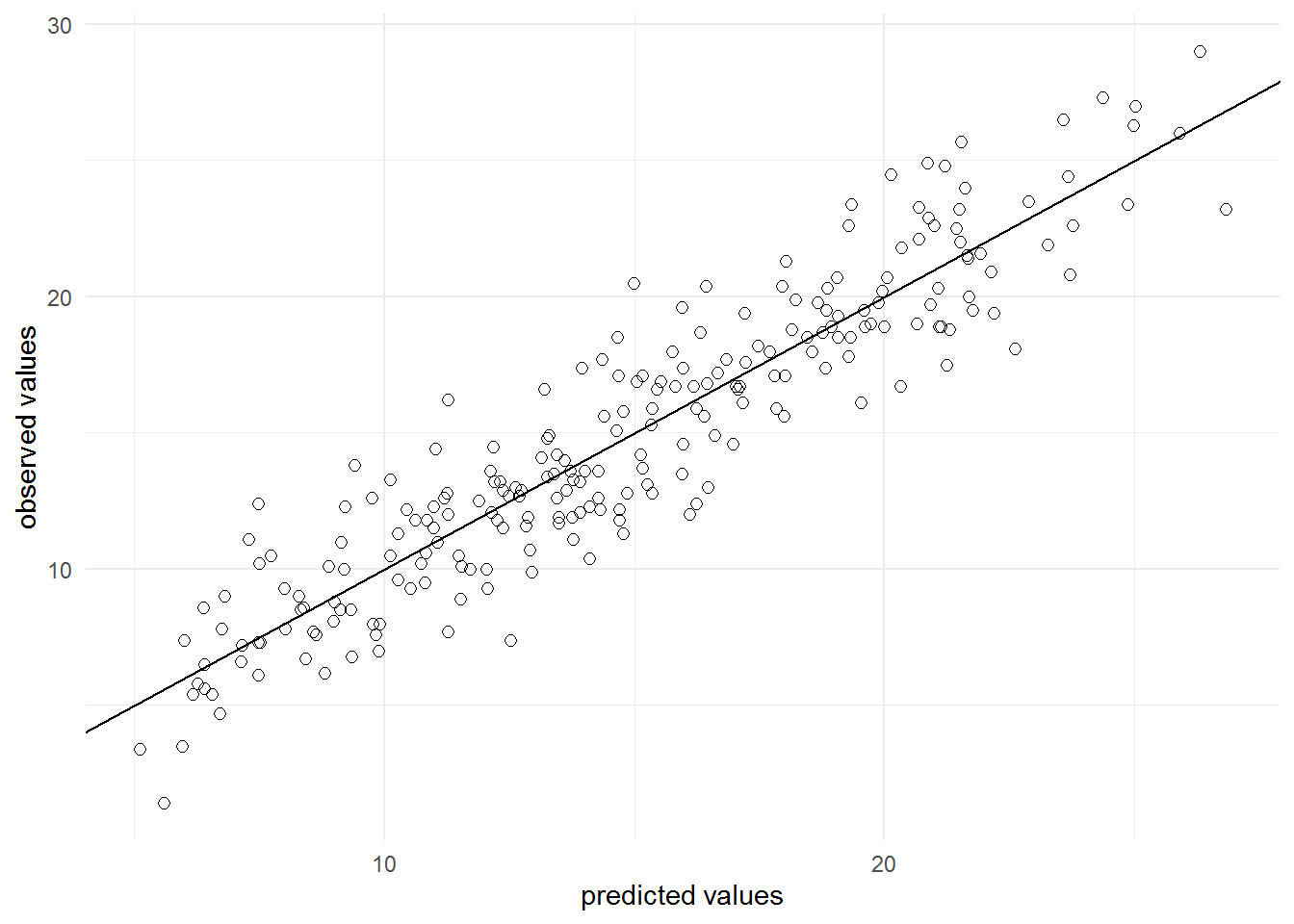
In addition, the output tells us that our predictions on average deviate from the observed values by 2048 units (see residual standard error, remember that the sales variable is measures in thousand units).
Of course, you could have also used the functions included in the ggstatsplot package to report the results from your regression model.
ggcoefstats(x = linear_model, k = 3, title = "Sales predicted by TV-, online-, & radio advertising")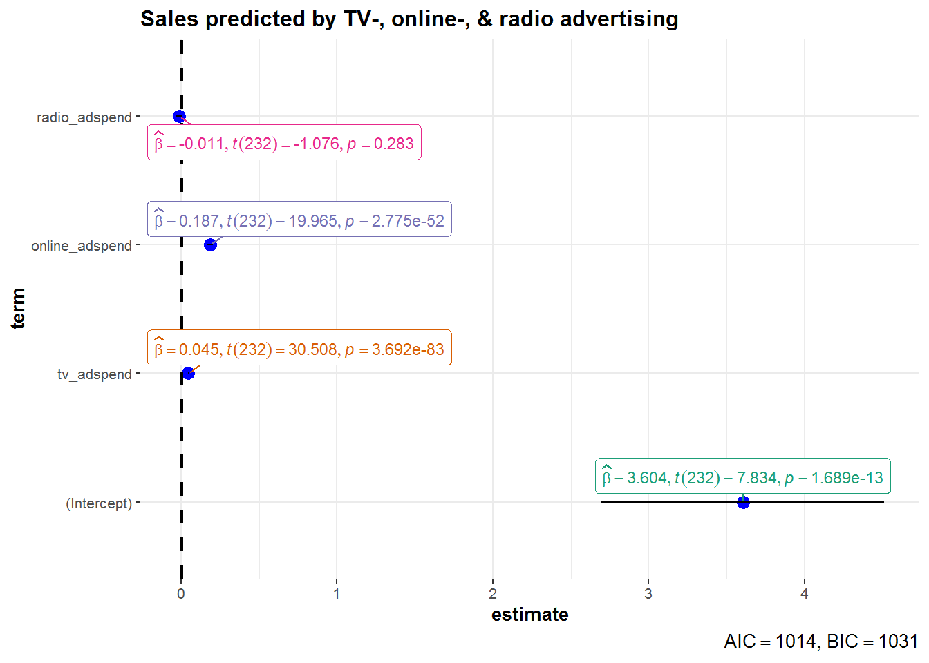
9.2.4 Q4
Finally, we can predict the outcome for the given marketing mix using the following equation:
\[\hat{Sales} = \beta_0 + \beta_1*150 + \beta_2*26 + \beta_3*15 \]
The coefficients can be extracted from the summary of the linear model and used for quick sales value prediction as follows:
summary(linear_model)$coefficients[1, 1] + summary(linear_model)$coefficients[2,
    1] * 150 + summary(linear_model)$coefficients[3,
    1] * 26 + summary(linear_model)$coefficients[4,
    1] * 15
## [1] 15.11236\[\hat{sales}= 3.6 + 0.045*150 + 0.187*26 + 0.011*15 = 15.11\]
This means that given the planned marketing mix, we would expect to sell around 15,112 units.