My Cool Title

An example

Level 1 Headline

Here I want to cite Golder et al. (2022). Maybe I want to cite them in brackets (Golder et al. 2022) or (see Golder et al. 2022, 12). The references are stored in the references.bib file and follow the BibTeX format. You can find BibTeX entries for most papers on google scholar. Below the search entry is a “Cite” button which opens a pop-up that has a “BibTeX” link (e.g., here).

Links to websites can be added to your document with [LINK TEXT](https://example.com).

Level 2 Headline

R code goes into code chunks. Chunk options are set with a special comment #|. Here we added echo: fenced and code-fold: false to show the code but you typically want to remove those from the options:

```{r}
#| code-fold: false
library(ggplot2)
ggplot(data.frame(x=rnorm(100), y=rnorm(100)), aes(x,y)) +
    geom_point() +
    theme_minimal()
```

Special comments are useful to control output size and captions for images and prevent R from printing warnings (warning: false):

```{r}
#| code-fold: false
#| fig-cap: "Very cool correlation"
#| fig-width: 4
#| fig-height: 4
#| warning: false
library(palmerpenguins)
ggplot(penguins, aes(x = body_mass_g, y = bill_length_mm)) +
    geom_point() +
    geom_smooth(method="lm") +
    theme_minimal()
```

Very cool correlation

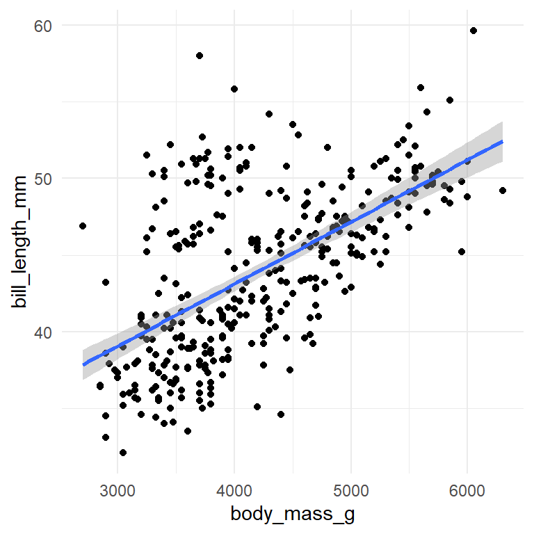
Here is the data

Code

penguins

Another main section

You can use R code inline e.g., to print summary statistics automatically. You could say the average body mass of a penguin in the Palmer Penguins dataset is 4201.8g (`round(mean(penguins$body_mass_g, na.rm=TRUE), digits=1)`).

See the quarto documentation for more info.

HTML tables

Summary statistics

Code

library(dplyr)
library(gt)
penguins |>
    group_by(island, species) |>
    select(-year) |>
    summarize_if(is.numeric, \(v)mean(v, na.rm=TRUE)) |>
    gt(rowname_col = "species") |>
    tab_header(
        title = "Penguins",
        subtitle = "Average by Island and Species"
    ) |>
    fmt_number(
        columns = bill_length_mm:flipper_length_mm,
        pattern = "{x}mm",
        decimals = 1
    ) |>
    fmt_number(
        columns = body_mass_g,
        suffixing = "KG",
        decimals = 1
    ) |>
    tab_spanner(
        label = "Bill",
        columns = bill_length_mm:bill_depth_mm
    ) |>
    cols_label(
        bill_length_mm = "length",
        bill_depth_mm = "depth",
        flipper_length_mm = "flipper length",
        body_mass_g = "body mass"
    )

Penguins
Average by Island and Species
	Bill		flipper length	body mass
	length	depth
Biscoe
Adelie	39.0mm	18.4mm	188.8mm	3.7KG
Gentoo	47.5mm	15.0mm	217.2mm	5.1KG
Dream
Adelie	38.5mm	18.3mm	189.7mm	3.7KG
Chinstrap	48.8mm	18.4mm	195.8mm	3.7KG
Torgersen
Adelie	39.0mm	18.4mm	191.2mm	3.7KG

Regression Tables

Code

library(modelsummary)
library(fixest)
## species and year fixed effects with SE clustered by species
## Note that this is JUST for presentation purposes
## and not a meaningful model!!!
mod1 <- feols(
    body_mass_g ~ flipper_length_mm + bill_length_mm | species + year,
    data = penguins
)
mod2 <-  feols(
    body_mass_g ~ flipper_length_mm + bill_length_mm + bill_depth_mm | species + year,
    data = penguins
)
mod3 <-  feols(
    body_mass_g ~ flipper_length_mm + bill_length_mm + bill_depth_mm | species,
    cluster = ~species,
    data = penguins
)
mod4 <- lm(
    body_mass_g ~ flipper_length_mm + bill_length_mm + bill_depth_mm + species,
    data = penguins
)
modelsummary(
    list(`no depth` = mod1, 
         `with depth` = mod2,
         `species FE` = mod3,
         `species dummy` = mod4),
    coef_map = c(
        "flipper_length_mm" = "flipper length",
        "bill_length_mm" = "bill length",
        "bill_depth_mm" = "bill depth",
        "speciesChinstrap" = "Chinstrap vs. Adelie",
        "speciesGentoo" = "Gentoo vs. Adelie"
    ),
    gof_map = c(
        "nobs", 
        "r.squared", 
        "r2.within", 
        "FE: species", 
        "FE: year", 
        "vcov.type"),
    vcov = ~species,
    title = "Modelling Penguin Body Mass",
    notes = "OLS with species dummy results in the same parameters as species FE but is less efficient",
    output = "gt"
) |>
    tab_spanner(columns = 2:4, label = "Fixed Effects") |>
    tab_spanner(columns = 5, label = "OLS")

Modelling Penguin Body Mass

	Fixed Effects			OLS
	no depth	with depth	species FE	species dummy
flipper length	30.892	22.500	20.241	20.241
	(3.999)	(3.853)	(2.690)	(2.698)
bill length	60.053	42.298	41.468	41.468
	(13.244)	(12.217)	(11.604)	(11.638)
bill depth		131.265	140.328	140.328
		(16.878)	(16.141)	(16.189)
Chinstrap vs. Adelie				-513.247
				(108.516)
Gentoo vs. Adelie				934.887
				(24.742)
Num.Obs.	342	342	342	342
R2	0.829	0.849	0.847	0.847
R2 Within	0.482	0.544	0.537
Std.Errors	by: species	by: species	by: species	by: species
FE: species	X	X	X
FE: year	X	X
OLS with species dummy results in the same parameters as species FE but is less efficient

References

Golder, Peter N, Marnik G Dekimpe, Jake T An, Harald J van Heerde, Darren SU Kim, and Joseph W Alba. 2022. “Learning from Data: An Empirics-First Approach to Relevant Knowledge Generation.” Journal of Marketing.