Difference in Differences Workshop

UNSW Data Science Hub

Preliminaries

This tutorial uses the R statistical software (R Core Team 2022) and assumes you have a recent version with the standard packages loaded (this is the case in a fresh installation without modifications).

Code

library(ggplot2)
library(psych)
library(data.table)
library(tidyverse)
options(scipen = 999)
# panel data models
#-------------------------------------------------------------------
# load data
music_data <- fread("https://raw.githubusercontent.com/WU-RDS/RMA2022/main/data/music_data.csv")
# convert to factor
music_data$song_id <- as.factor(music_data$song_id)
music_data$genre <- as.factor(music_data$genre)
music_data

Code

# example plot to visualize the data structure
ggplot(music_data, aes(x = week, y = streams / 1000000, group = song_id, fill = song_id, color = song_id)) +
    geom_area(position = "stack", alpha = 0.65) +
    labs(x = "Week", y = "Total streams (in million)", title = "Weekly number of streams by song") +
    theme_bw() +
    theme(plot.title = element_text(hjust = 0.5, color = "#666666"), legend.position = "none")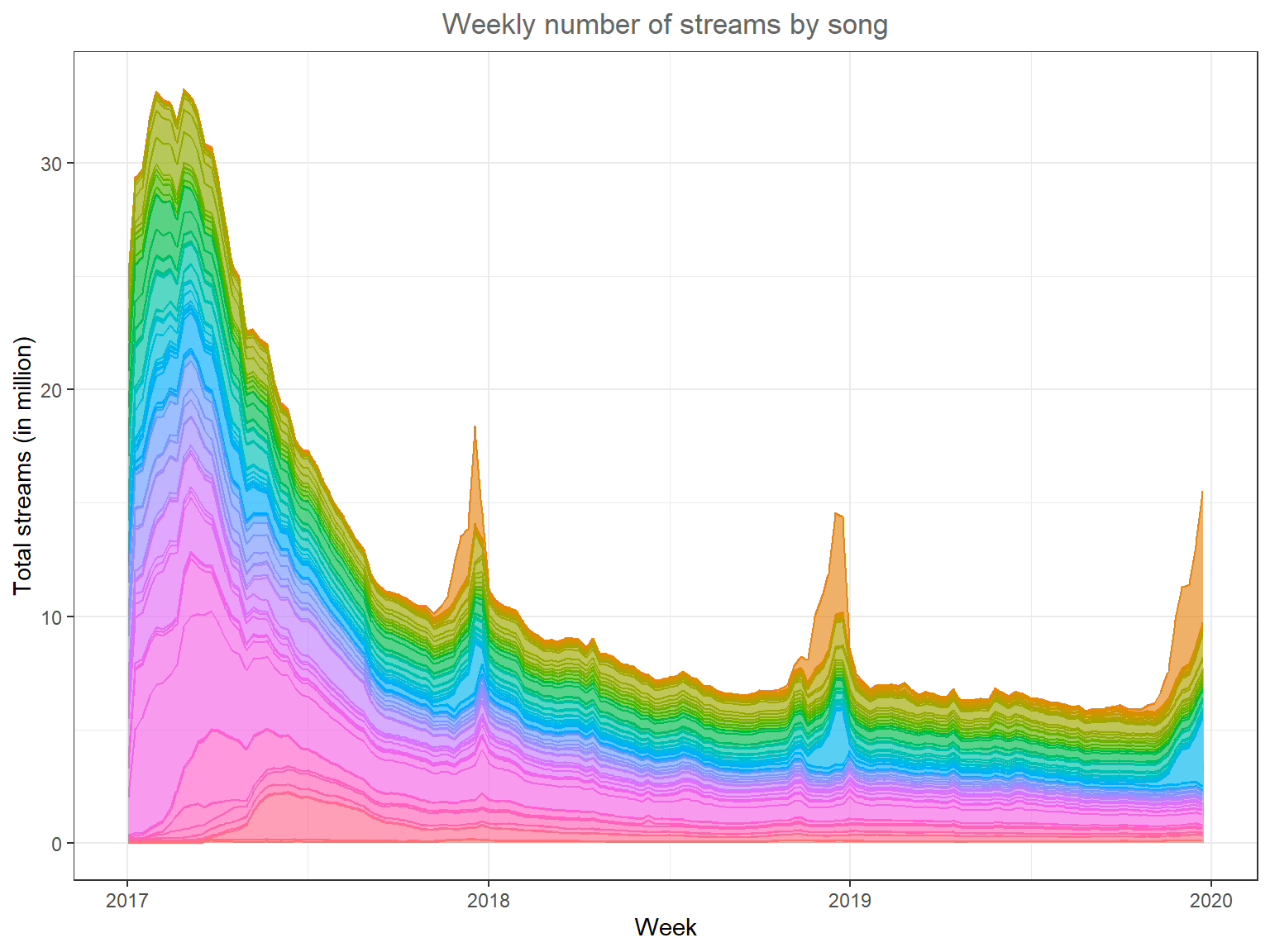

Baseline model

Estimation of different specifications of a linear model using OLS (without fixed effects). The lm command for OLS estimation is available in your R session by default.

Code

# estimate the baseline model
fe_m0 <- lm(log(streams) ~ log(radio + 1) + log(adspend + 1),
    data = music_data
)

# ... + control for song age
fe_m1 <- lm(log(streams) ~ log(radio + 1) + log(adspend + 1) + log(weeks_since_release + 1),
    data = music_data
)

# ... + playlist follower variable
fe_m2 <- lm(log(streams) ~ log(radio + 1) + log(adspend + 1) + log(weeks_since_release + 1) + log(playlist_follower),
    data = music_data
)

# ... + song fixed effects
fe_m3 <- lm(
    log(streams) ~ log(radio + 1) + log(adspend + 1) + log(playlist_follower) + log(weeks_since_release + 1) +
        as.factor(song_id),
    data = music_data
)
library(stargazer)
stargazer(fe_m0, fe_m1, fe_m2, fe_m3, type = "html")

	Dependent variable:
	log(streams)
	(1)	(2)	(3)	(4)
log(radio + 1)	0.542***	0.503***	0.280***	0.107***
	(0.012)	(0.013)	(0.010)	(0.004)
log(adspend + 1)	0.033***	0.035***	0.056***	0.022***
	(0.011)	(0.011)	(0.008)	(0.003)
log(weeks_since_release + 1)		-0.143***	0.074***	-0.400***
		(0.014)	(0.010)	(0.008)
as.factor(song_id)2				0.918***
				(0.051)
as.factor(song_id)3				0.026
				(0.051)
as.factor(song_id)4				1.257***
				(0.050)
as.factor(song_id)5				-0.336***
				(0.051)
as.factor(song_id)6				0.648***
				(0.051)
as.factor(song_id)7				2.641***
				(0.061)
as.factor(song_id)8				3.802***
				(0.052)
as.factor(song_id)9				3.960***
				(0.051)
as.factor(song_id)10				3.812***
				(0.054)
as.factor(song_id)11				2.681***
				(0.055)
as.factor(song_id)12				4.046***
				(0.052)
as.factor(song_id)13				2.976***
				(0.050)
as.factor(song_id)14				0.727***
				(0.053)
as.factor(song_id)15				4.031***
				(0.050)
as.factor(song_id)16				4.032***
				(0.054)
as.factor(song_id)17				4.422***
				(0.052)
as.factor(song_id)18				0.915***
				(0.052)
as.factor(song_id)19				2.971***
				(0.050)
as.factor(song_id)20				2.334***
				(0.061)
as.factor(song_id)21				4.930***
				(0.053)
as.factor(song_id)22				3.401***
				(0.057)
as.factor(song_id)23				3.040***
				(0.060)
as.factor(song_id)24				2.695***
				(0.060)
as.factor(song_id)25				1.229***
				(0.050)
as.factor(song_id)26				4.313***
				(0.052)
as.factor(song_id)27				3.514***
				(0.055)
as.factor(song_id)28				1.026***
				(0.055)
as.factor(song_id)29				4.440***
				(0.051)
as.factor(song_id)30				2.444***
				(0.062)
as.factor(song_id)31				0.615***
				(0.055)
as.factor(song_id)32				1.218***
				(0.054)
as.factor(song_id)33				-0.246***
				(0.052)
as.factor(song_id)34				3.587***
				(0.055)
as.factor(song_id)35				4.965***
				(0.054)
as.factor(song_id)36				1.904***
				(0.053)
as.factor(song_id)37				1.255***
				(0.054)
as.factor(song_id)38				2.409***
				(0.062)
as.factor(song_id)39				0.375***
				(0.053)
as.factor(song_id)40				2.616***
				(0.050)
as.factor(song_id)41				0.803***
				(0.053)
as.factor(song_id)42				1.569***
				(0.054)
as.factor(song_id)43				2.041***
				(0.053)
as.factor(song_id)44				1.517***
				(0.051)
as.factor(song_id)45				2.792***
				(0.064)
as.factor(song_id)46				3.707***
				(0.051)
as.factor(song_id)47				2.526***
				(0.061)
as.factor(song_id)48				2.781***
				(0.051)
as.factor(song_id)49				1.731***
				(0.054)
as.factor(song_id)50				1.655***
				(0.058)
as.factor(song_id)51				2.293***
				(0.061)
as.factor(song_id)52				0.406***
				(0.052)
as.factor(song_id)53				2.113***
				(0.060)
as.factor(song_id)54				3.615***
				(0.051)
as.factor(song_id)55				3.393***
				(0.052)
as.factor(song_id)56				1.346***
				(0.056)
as.factor(song_id)57				2.891***
				(0.056)
as.factor(song_id)58				2.277***
				(0.052)
as.factor(song_id)59				1.621***
				(0.056)
as.factor(song_id)60				3.518***
				(0.059)
as.factor(song_id)61				0.906***
				(0.051)
as.factor(song_id)62				1.741***
				(0.058)
as.factor(song_id)63				2.100***
				(0.052)
as.factor(song_id)64				2.151***
				(0.060)
as.factor(song_id)65				0.438***
				(0.051)
as.factor(song_id)66				3.008***
				(0.059)
as.factor(song_id)67				2.116***
				(0.063)
as.factor(song_id)68				2.413***
				(0.061)
as.factor(song_id)69				2.247***
				(0.053)
as.factor(song_id)70				2.829***
				(0.059)
as.factor(song_id)71				2.523***
				(0.055)
as.factor(song_id)72				-0.802***
				(0.051)
as.factor(song_id)73				2.950***
				(0.059)
as.factor(song_id)74				1.618***
				(0.051)
as.factor(song_id)75				3.039***
				(0.055)
as.factor(song_id)76				4.060***
				(0.051)
as.factor(song_id)77				4.201***
				(0.053)
as.factor(song_id)78				2.814***
				(0.062)
as.factor(song_id)79				3.514***
				(0.051)
as.factor(song_id)80				1.954***
				(0.056)
as.factor(song_id)81				2.912***
				(0.062)
as.factor(song_id)82				3.188***
				(0.065)
as.factor(song_id)83				2.051***
				(0.053)
as.factor(song_id)84				0.161***
				(0.051)
as.factor(song_id)85				-0.172***
				(0.052)
as.factor(song_id)86				2.882***
				(0.060)
as.factor(song_id)87				2.757***
				(0.051)
as.factor(song_id)88				3.023***
				(0.058)
as.factor(song_id)89				3.063***
				(0.062)
as.factor(song_id)90				1.302***
				(0.053)
as.factor(song_id)91				2.458***
				(0.062)
as.factor(song_id)92				1.426***
				(0.054)
as.factor(song_id)93				0.672***
				(0.051)
as.factor(song_id)94				2.901***
				(0.062)
as.factor(song_id)95				0.710***
				(0.052)
as.factor(song_id)96				0.944***
				(0.058)
as.factor(song_id)97				4.557***
				(0.052)
log(playlist_follower)			0.536***	0.439***
			(0.005)	(0.006)
Constant	10.091***	10.800***	2.530***	3.938***
	(0.015)	(0.070)	(0.091)	(0.083)
Observations	15,132	15,132	15,132	15,132
R2	0.130	0.136	0.524	0.945
Adjusted R2	0.130	0.136	0.523	0.944
Residual Std. Error	1.734 (df = 15129)	1.728 (df = 15128)	1.283 (df = 15127)	0.439 (df = 15031)
F Statistic	1,129.772*** (df = 2; 15129)	794.258*** (df = 3; 15128)	4,156.097*** (df = 4; 15127)	2,564.991*** (df = 100; 15031)
Note:	p<0.1; p<0.05; p<0.01

Fixed Effects model

Estimation of a linear model with song and song-time fixed effects using the fixest (Bergé 2018) package. Note that this package also implements the estimator proposed by Sun and Abraham (2020) for staggered adoption (see ?sunab).

Code

# ... same as m3 using the fixest package
library(fixest) # https://lrberge.github.io/fixest/
fe_m4 <- feols(
    log(streams) ~ log(radio + 1) + log(adspend + 1) + log(playlist_follower) + log(weeks_since_release + 1) |
        song_id,
    data = music_data
)
# ... + week fixed effects
fe_m5 <- feols(
    log(streams) ~ log(radio + 1) + log(adspend + 1) + log(playlist_follower) + log(weeks_since_release + 1) |
        song_id + week,
    data = music_data
)
etable(fe_m4, fe_m5, se = "cluster")

Code

# extract fixed effects coefficients
fixed_effects <- fixef(fe_m5)
summary(fixed_effects)

Fixed_effects coefficients
                        song_id  week
Number of fixed-effects      97   156
Number of references          0     1
Mean                       6.37 0.688
Standard-deviation         1.37 0.161

COEFFICIENTS:
  song_id:     1     2     3    4    5                 
           4.188 5.041 4.061 5.27 3.66 ... 92 remaining
-----
  week: 2017-01-02 2017-01-09 2017-01-16 2017-01-23 2017-01-30
                 0     0.0499    0.06933      0.171      0.221
                   
  ... 151 remaining

Code

plot(fixed_effects)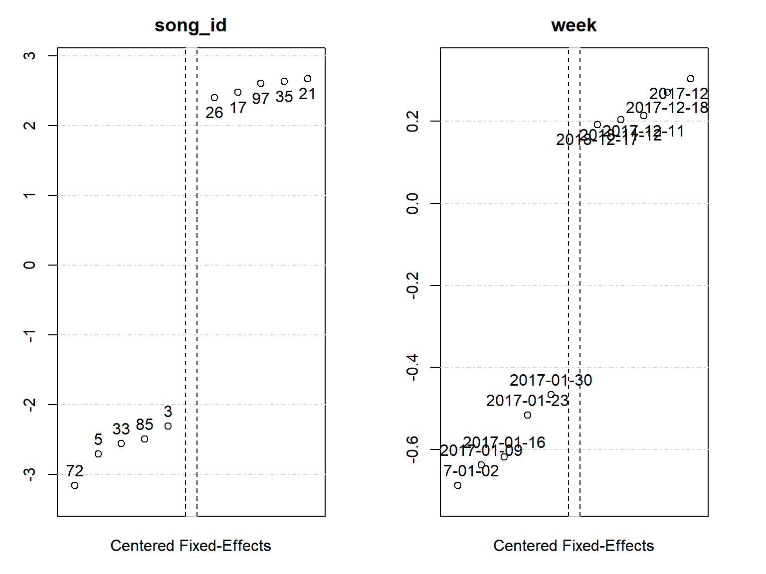

Mixed Effects model

Danger

The term Fixed Effects is not used consistently in the literature. Here we view fixed effects as unit level constants (R packages: fixest, lfe, or alpaca). If you find the term “fixed effects” in the context of “mixed effects models” or “random effects models” (in R when the lme4 package is used) it refers to coefficients that are fixed across units.

Estimation of mixed effects model using lme4. This allows explicitly modelling heterogeneity of intercept and slopes across units.

Code

library(lme4) # https://github.com/lme4/lme4
music_data$log_playlist_follower <- log(music_data$playlist_follower)
music_data$log_streams <- log(music_data$streams)
re_m1 <- lmer(log_streams ~ log(radio + 1) + log(adspend + 1) + log_playlist_follower + log(weeks_since_release + 1) + (1 + log_playlist_follower | song_id), data = music_data)
summary(re_m1)

Linear mixed model fit by REML ['lmerMod']
Formula: 
log_streams ~ log(radio + 1) + log(adspend + 1) + log_playlist_follower +  
    log(weeks_since_release + 1) + (1 + log_playlist_follower |      song_id)
   Data: music_data

REML criterion at convergence: 14776.3

Scaled residuals: 
    Min      1Q  Median      3Q     Max 
-8.4922 -0.3578 -0.0084  0.3620 13.7550 

Random effects:
 Groups   Name                  Variance Std.Dev. Corr 
 song_id  (Intercept)           26.467   5.1446        
          log_playlist_follower  0.140   0.3742   -0.95
 Residual                        0.144   0.3794        
Number of obs: 15132, groups:  song_id, 97

Fixed effects:
                              Estimate Std. Error t value
(Intercept)                   6.369815   0.537152   11.86
log(radio + 1)                0.084025   0.004081   20.59
log(adspend + 1)              0.026216   0.002496   10.50
log_playlist_follower         0.446280   0.038877   11.48
log(weeks_since_release + 1) -0.478857   0.008095  -59.16

Correlation of Fixed Effects:
            (Intr) lg(r+1) lg(d+1) lg_pl_
log(radi+1)  0.051                       
lg(dspnd+1)  0.011 -0.126                
lg_plylst_f -0.952 -0.073  -0.013        
lg(wks__+1) -0.076  0.382   0.043   0.000

Code

library(sjPlot)
plot_model(re_m1, show.values = TRUE, value.offset = .3)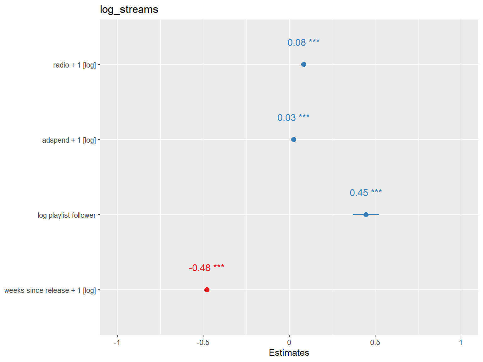

Code

# plot random-slope-intercept
plot_model(re_m1,
    type = "pred", terms = c("log_playlist_follower", "song_id"),
    pred.type = "re", ci.lvl = NA
) +
    scale_colour_manual(values = hcl(0, 100, seq(40, 100, length = 97))) +
    theme(legend.position = "bottom", legend.key.size = unit(0.3, "cm")) + guides(colour = guide_legend(nrow = 5))

Difference-in-Differences estimator

“Canonical” Diff-in-Diff

Data preparation using the data.table and dplyr packages.

Code

# load data
did_data <- fread("https://raw.github.com/WU-RDS/RMA2022/main/data/did_data_exp.csv")
# pre-processing
did_data$song_id <- as.character(did_data$song_id)
did_data$treated_fct <- factor(did_data$treated, levels = c(0, 1), labels = c("non-treated", "treated"))
did_data$post_fct <- factor(did_data$post, levels = c(0, 1), labels = c("pre", "post"))
did_data$week <- as.Date(did_data$week)
did_data <- did_data %>%
    dplyr::filter(!song_id %in% c("101", "143", "154", "63", "161", "274")) %>%
    as.data.frame()
did_data

Number of songs by treatment status:

Code

library(gt)
did_data %>%
    dplyr::group_by(treated) %>%
    dplyr::summarise(unique_songs = n_distinct(song_id)) |>
    gt()

treated	unique_songs
0	231
1	53

Visualization of the panel structure using the panelView package.

Code

head(did_data)

Code

did_data %>%
    dplyr::group_by(treated) %>%
    dplyr::summarise(unique_songs = n_distinct(song_id))

Code

library(panelView) # https://yiqingxu.org/packages/panelview/
panelview(streams ~ treated_post, data = did_data, index = c("song_id", "week"), pre.post = TRUE, by.timing = TRUE, axis.lab.angle = 90)

Code

panelview(streams ~ treated_post, data = did_data, index = c("song_id", "week"), type = "outcome", axis.lab.angle = 90)

Code

did_data <- did_data %>%
    group_by(song_id) %>%
    dplyr::mutate(mean_streams = mean(streams)) %>%
    as.data.frame()
panelview(streams ~ treated_post, data = did_data %>% dplyr::filter(mean_streams < 70000), index = c("song_id", "week"), type = "outcome", axis.lab.angle = 90)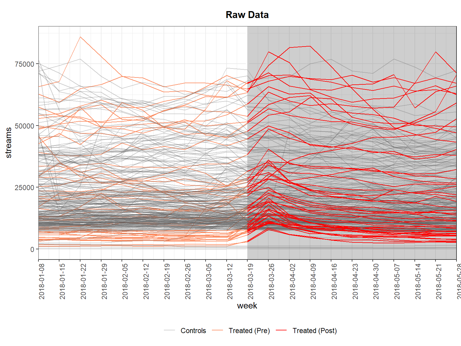

Visualization of the outcome variable by treatment group using the ggplot2 package.

Code

# alternatively, split plot by group
# compute the mean streams per group and week
did_data <- did_data %>%
    dplyr::group_by(treated_fct, week) %>%
    dplyr::mutate(mean_streams_grp = mean(log(streams))) %>%
    as.data.frame()
# set color scheme for songs
cols <- c(rep("gray", length(unique(did_data$song_id))))
# set labels for axis
abbrev_x <- c(
    "-10", "", "-8", "",
    "-6", "", "-4", "",
    "-2", "", "0",
    "", "+2", "", "+4",
    "", "+6", "", "+8",
    "", "+10"
)
# axis titles and names
title_size <- 24
font_size <- 14
line_size <- 1 / 2
# create plot
ggplot(did_data) +
    geom_step(aes(x = week, y = log(streams), color = song_id), alpha = 0.75) +
    geom_step(aes(x = week, y = mean_streams_grp), color = "black", size = 2, alpha = 0.5) +
    # geom_vline(xintercept = as.Date("2018-03-19"),color="black",linetype="dashed") +
    labs(
        x = "week before/after playlist listing", y = "ln(streams)",
        title = "Number of weekly streams per song"
    ) +
    scale_color_manual(values = cols) +
    theme_bw() +
    scale_x_continuous(breaks = unique(did_data$week), labels = abbrev_x) +
    theme(
        legend.position = "none",
        panel.grid.minor.x = element_blank(),
        panel.grid.major.x = element_blank(),
        strip.text.x = element_text(size = font_size),
        panel.grid.major.y = element_line(
            color = "gray75",
            size = 0.25,
            linetype = 1
        ),
        panel.grid.minor.y = element_line(
            color = "gray75",
            size = 0.25,
            linetype = 1
        ),
        plot.title = element_text(color = "#666666", size = title_size),
        axis.title = element_text(size = font_size),
        axis.text = element_text(size = font_size),
        plot.subtitle = element_text(color = "#666666", size = font_size),
        axis.text.x = element_text(size = font_size)
    ) +
    facet_wrap(~treated_fct)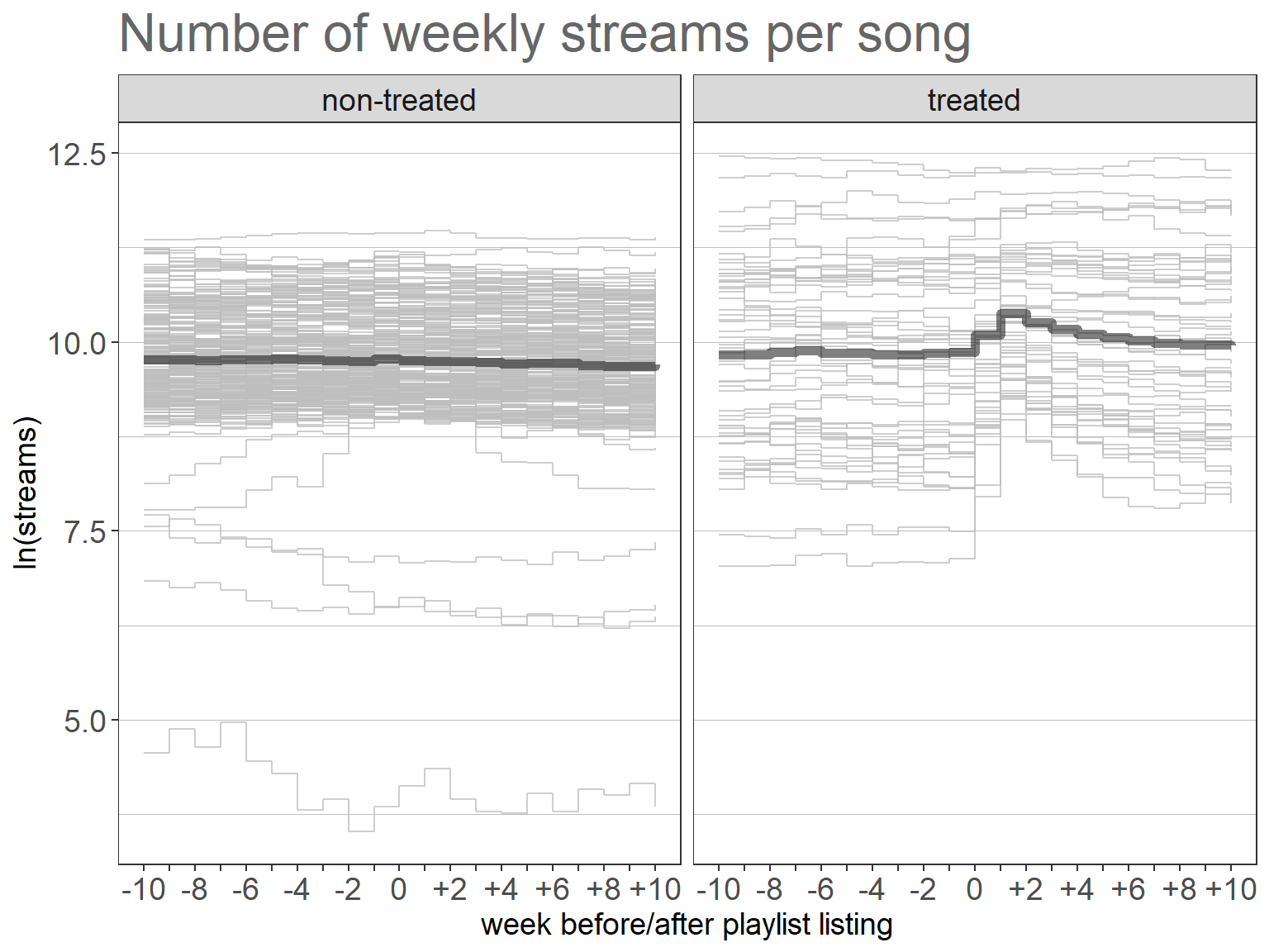

Baseline model

Estimation of the baseline model using dummy-variables for the post-treatment period (\(1\) for all units in the post-treatment period) and the treatment group (always \(1\) for units that are eventually treated) as well as their interaction. The coefficient of the latter is the difference-in-differences estimator of the treatment effect.

Code

# run baseline did model
did_m1 <- lm(log(streams + 1) ~ treated * post,
    data = did_data %>% dplyr::filter(week != as.Date("2018-03-19"))
)
stargazer(did_m1, type = "html")

	Dependent variable:
	log(streams + 1)
treated	0.086**
	(0.041)
post	-0.053**
	(0.025)
treated:post	0.287***
	(0.058)
Constant	9.767***
	(0.018)
Observations	5,680
R2	0.015
Adjusted R2	0.014
Residual Std. Error	0.857 (df = 5676)
F Statistic	28.782*** (df = 3; 5676)
Note:	p<0.1; p<0.05; p<0.01

Two-Way Fixed Effects model

Alternative estimation of the same difference-in-differences parameter as above using unit-time fixed effects (fixest).

Code

# same model using fixed effects specification
did_m2 <- feols(
    log(streams + 1) ~ treated * post |
        song_id + week,
    cluster = "song_id",
    data = did_data %>% dplyr::filter(week != as.Date("2018-03-19"))
)
etable(did_m2, se = "cluster")

The did package

One of the most useful packages for the estimation of difference-in-differences with staggered adoption is did (Callaway and Sant’Anna 2021a). However the approach proposed by Callaway and Sant’Anna (2021b) also naturally extends to comparison of the canonical diff-in-diffs specification. First, group-time ATTs are calculated (in their paper group refers to adoption cohort). Second, the ATTs are aggregated using a group-size weighted average. Inference for this aggregate is implemented in the package.

Code

### DID PACKAGE
library(did)
## Treatment happens between period 10 & 11
## G is indicator of when a unit is treated
did_data$period <- as.numeric(factor(as.character(did_data$week),
    levels = as.character(sort(unique(did_data$week)))
))
did_data$log_streams <- log(did_data$streams + 1)
did_data$G <- 11 * did_data$treated
did_data$id <- as.numeric(did_data$song_id)

simple_gt_att <- att_gt(
    yname = "log_streams",
    tname = "period",
    idname = "id",
    gname = "G",
    data = did_data
)
## "simple" gives a weighted average of group-time effects weighted by group (treatment time) size
aggte(simple_gt_att, type = "simple")

Call:
aggte(MP = simple_gt_att, type = "simple")

Reference: Callaway, Brantly and Pedro H.C. Sant'Anna.  "Difference-in-Differences with Multiple Time Periods." Journal of Econometrics, Vol. 225, No. 2, pp. 200-230, 2021. <https://doi.org/10.1016/j.jeconom.2020.12.001>, <https://arxiv.org/abs/1803.09015> 

    ATT    Std. Error     [ 95%  Conf. Int.]  
 0.2813        0.0401     0.2028      0.3599 *


---
Signif. codes: `*' confidence band does not cover 0

Control Group:  Never Treated,  Anticipation Periods:  0
Estimation Method:  Doubly Robust

Parallel trends assessment

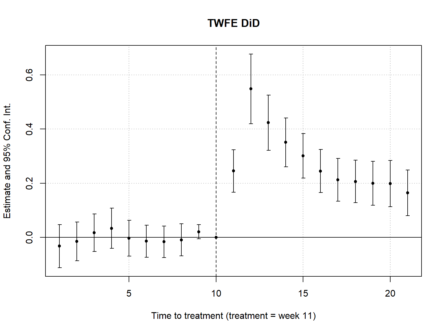
Period-specific effects

Conduct leads & lags analysis to assess “pre-trends” using fixest. \(H_0\) should not be rejected pre-treatment.

Code

did_data <- did_data %>%
    dplyr::group_by(song_id) %>%
    dplyr::mutate(period = seq(n())) %>%
    as.data.frame()
did_m3 <- fixest::feols(log(streams) ~ i(period, treated, ref = 10) | song_id + period,
    cluster = "song_id",
    data = did_data
)
etable(did_m3, se = "cluster")

Code

fixest::iplot(did_m3,
    xlab = "Time to treatment (treatment = week 11)",
    main = "TWFE DiD"
)

did provides a Wald test for pre-treatment trends.

Code

## for time < group these are pseudo ATTs -> pre-test for parallel trends
summary(simple_gt_att)

Call:
att_gt(yname = "log_streams", tname = "period", idname = "id", 
    gname = "G", data = did_data)

Reference: Callaway, Brantly and Pedro H.C. Sant'Anna.  "Difference-in-Differences with Multiple Time Periods." Journal of Econometrics, Vol. 225, No. 2, pp. 200-230, 2021. <https://doi.org/10.1016/j.jeconom.2020.12.001>, <https://arxiv.org/abs/1803.09015> 

Group-Time Average Treatment Effects:
 Group Time ATT(g,t) Std. Error [95% Simult.  Conf. Band]  
    11    2   0.0176     0.0157       -0.0234      0.0586  
    11    3   0.0316     0.0138       -0.0045      0.0677  
    11    4   0.0168     0.0161       -0.0251      0.0586  
    11    5  -0.0369     0.0130       -0.0708     -0.0030 *
    11    6  -0.0108     0.0153       -0.0508      0.0292  
    11    7  -0.0022     0.0105       -0.0296      0.0252  
    11    8   0.0070     0.0139       -0.0291      0.0432  
    11    9   0.0296     0.0305       -0.0499      0.1092  
    11   10  -0.0200     0.0138       -0.0559      0.0159  
    11   11   0.2449     0.0412        0.1376      0.3523 *
    11   12   0.5485     0.0658        0.3769      0.7202 *
    11   13   0.4236     0.0535        0.2842      0.5630 *
    11   14   0.3508     0.0481        0.2254      0.4762 *
    11   15   0.3010     0.0429        0.1892      0.4127 *
    11   16   0.2445     0.0408        0.1381      0.3509 *
    11   17   0.2123     0.0410        0.1055      0.3191 *
    11   18   0.2063     0.0411        0.0990      0.3135 *
    11   19   0.1994     0.0427        0.0881      0.3108 *
    11   20   0.1988     0.0437        0.0849      0.3127 *
    11   21   0.1646     0.0434        0.0513      0.2778 *
---
Signif. codes: `*' confidence band does not cover 0

P-value for pre-test of parallel trends assumption:  0.12298
Control Group:  Never Treated,  Anticipation Periods:  0
Estimation Method:  Doubly Robust

Code

ggdid(simple_gt_att)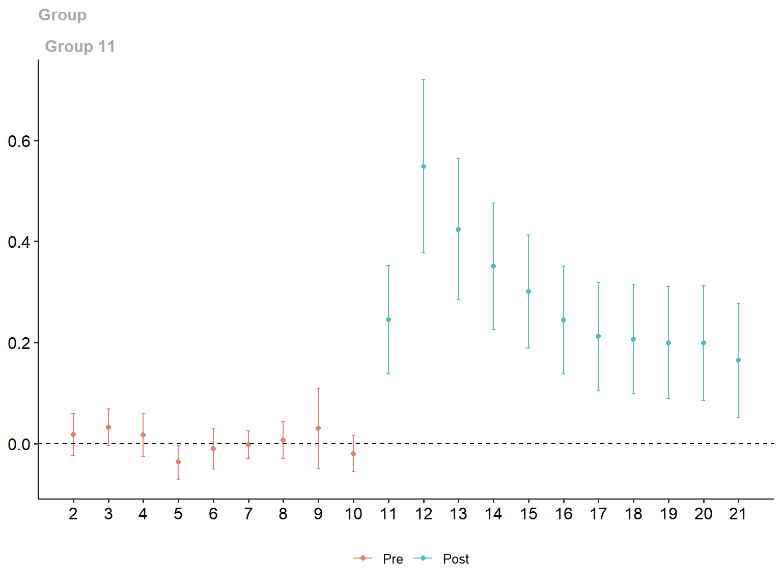

Placebo-test

Code

did_data_placebo <- did_data %>%
    dplyr::filter(period < 11) %>%
    as.data.frame()
did_data_placebo$post <- ifelse(did_data_placebo$period >= 5, 1, 0)
placebo_model <- feols(
    log(streams + 1) ~ treated * post |
        song_id + week,
    cluster = "song_id",
    data = did_data_placebo
)
etable(placebo_model, se = "cluster")

Sensitivity analysis

Rambachan and Roth (2023) propose (among other things) to test the robustness of the results to violations of the parallel trends in the post-treatment period relative to the pre-treatment period. We can check statistical significance of causale parameters if we impose that the post-treatment violation of parallel trends is not more than \(\bar M\) longer than the worst pre-treatment violation of parallel trends for different values of \(\bar M\).

Code

##### - honest pre-treatment trend assessment; https://github.com/asheshrambachan/HonestDiD
library(Rglpk)
library(HonestDiD)
betahat <- summary(did_m3)$coefficients # save the coefficients
sigma <- summary(did_m3)$cov.scaled # save the covariance matrix
## significant result is robust to allowing for violations of parallel trends
## up to >twice as big as the max violation in the pre-treatment period.
HonestDiD::createSensitivityResults_relativeMagnitudes(
    betahat = betahat, # coefficients
    sigma = sigma, # covariance matrix
    numPrePeriods = 10, # num. of pre-treatment coefs
    numPostPeriods = 10, # num. of post-treatment coefs
    Mbarvec = seq(0.5, 2.5, by = 0.5) # values of Mbar
)

Conditional parallel trends

Using did we can also estimate a model in which the trends are only parallel conditional on covariates by specifying the xformla argument.

Code

## Conditional pre-test
set.seed(123)
did_data$genre <- as.factor(did_data$genre)
conditional_gt_att <- att_gt(
    yname = "log_streams",
    tname = "period",
    idname = "id",
    gname = "G",
    xformla = ~genre,
    data = did_data
)
ggdid(conditional_gt_att)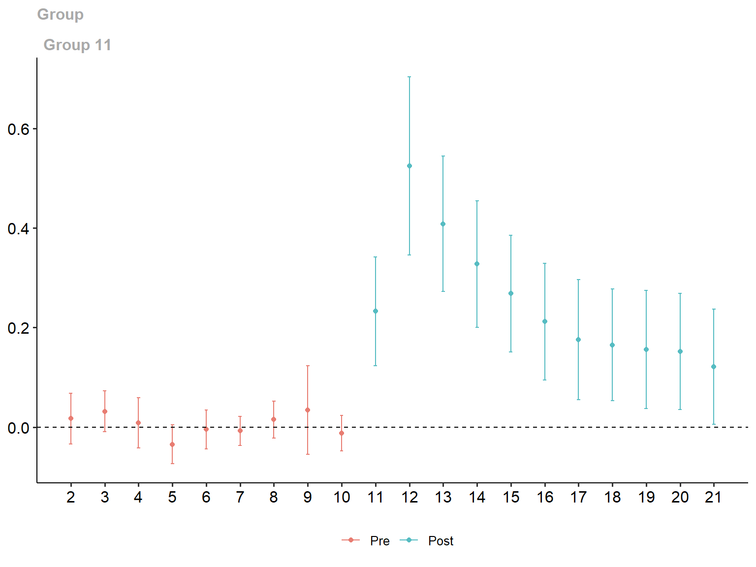

Code

summary(conditional_gt_att)

Call:
att_gt(yname = "log_streams", tname = "period", idname = "id", 
    gname = "G", xformla = ~genre, data = did_data)

Reference: Callaway, Brantly and Pedro H.C. Sant'Anna.  "Difference-in-Differences with Multiple Time Periods." Journal of Econometrics, Vol. 225, No. 2, pp. 200-230, 2021. <https://doi.org/10.1016/j.jeconom.2020.12.001>, <https://arxiv.org/abs/1803.09015> 

Group-Time Average Treatment Effects:
 Group Time ATT(g,t) Std. Error [95% Simult.  Conf. Band]  
    11    2   0.0169     0.0182       -0.0339      0.0677  
    11    3   0.0316     0.0147       -0.0093      0.0726  
    11    4   0.0085     0.0181       -0.0420      0.0591  
    11    5  -0.0346     0.0140       -0.0737      0.0046  
    11    6  -0.0047     0.0139       -0.0435      0.0341  
    11    7  -0.0075     0.0104       -0.0366      0.0215  
    11    8   0.0149     0.0131       -0.0217      0.0515  
    11    9   0.0345     0.0319       -0.0545      0.1235  
    11   10  -0.0123     0.0126       -0.0475      0.0229  
    11   11   0.2329     0.0392        0.1236      0.3423 *
    11   12   0.5249     0.0642        0.3459      0.7038 *
    11   13   0.4086     0.0487        0.2727      0.5445 *
    11   14   0.3276     0.0456        0.2003      0.4548 *
    11   15   0.2684     0.0421        0.1509      0.3859 *
    11   16   0.2119     0.0419        0.0949      0.3289 *
    11   17   0.1758     0.0433        0.0550      0.2965 *
    11   18   0.1651     0.0403        0.0528      0.2774 *
    11   19   0.1561     0.0426        0.0374      0.2748 *
    11   20   0.1519     0.0418        0.0354      0.2684 *
    11   21   0.1211     0.0414        0.0057      0.2366 *
---
Signif. codes: `*' confidence band does not cover 0

P-value for pre-test of parallel trends assumption:  0.16937
Control Group:  Never Treated,  Anticipation Periods:  0
Estimation Method:  Doubly Robust

Code

aggte(conditional_gt_att, type = "simple")

Call:
aggte(MP = conditional_gt_att, type = "simple")

Reference: Callaway, Brantly and Pedro H.C. Sant'Anna.  "Difference-in-Differences with Multiple Time Periods." Journal of Econometrics, Vol. 225, No. 2, pp. 200-230, 2021. <https://doi.org/10.1016/j.jeconom.2020.12.001>, <https://arxiv.org/abs/1803.09015> 

    ATT    Std. Error     [ 95%  Conf. Int.]  
 0.2495        0.0382     0.1746      0.3243 *


---
Signif. codes: `*' confidence band does not cover 0

Control Group:  Never Treated,  Anticipation Periods:  0
Estimation Method:  Doubly Robust

Heterogeneous treatment effects

Heterogeneity across groups

Estimation of treatment effect heterogeneity across genres using fixest.

Code

# heterogeneity across treated units
# example genre
did_m4 <- feols(
    log(streams + 1) ~ treated_post * as.factor(genre) |
        song_id + week,
    cluster = "song_id",
    data = did_data %>% dplyr::filter(week != as.Date("2018-03-19"))
)
etable(did_m4, se = "cluster")

Heterogeneity across time

Estimation of different treatment effects for multiple post-treatment periods using fixest.

Code

# heterogeneity across time
did_data$treated_post_1 <- ifelse(did_data$week > as.Date("2018-03-19") & did_data$week <= (as.Date("2018-03-19") + 21) & did_data$treated == 1, 1, 0)
did_data$treated_post_2 <- ifelse(did_data$week > as.Date("2018-04-09") & did_data$week <= (as.Date("2018-04-09") + 21) & did_data$treated == 1, 1, 0)
did_data$treated_post_3 <- ifelse(did_data$week > as.Date("2018-04-30") & did_data$treated == 1, 1, 0)
did_m5 <- feols(
    log(streams + 1) ~ treated_post_1 + treated_post_2 + treated_post_3 |
        song_id + week,
    cluster = "song_id",
    data = did_data %>% dplyr::filter(week != as.Date("2018-03-19"))
)
etable(did_m5, se = "cluster")

Again, the aggregation scheme in did can be used to get an equivalent estimator using the methodology proposed in Callaway and Sant’Anna (2021b).

Code

t_post_1 <- aggte(simple_gt_att, "dynamic", min_e = 1, max_e = 3)
t_post_2 <- aggte(simple_gt_att, "dynamic", min_e = 4, max_e = 6)
t_post_3 <- aggte(simple_gt_att, "dynamic", min_e = 7)

data.frame(
    period = c("post 1", "post 2", "post 3"),
    att = c(t_post_1$overall.att, t_post_2$overall.att, t_post_3$overall.att),
    se = c(t_post_1$overall.se, t_post_2$overall.se, t_post_3$overall.se)
)

Code

t_post_1

Call:
aggte(MP = simple_gt_att, type = "dynamic", min_e = 1, max_e = 3)

Reference: Callaway, Brantly and Pedro H.C. Sant'Anna.  "Difference-in-Differences with Multiple Time Periods." Journal of Econometrics, Vol. 225, No. 2, pp. 200-230, 2021. <https://doi.org/10.1016/j.jeconom.2020.12.001>, <https://arxiv.org/abs/1803.09015> 


Overall summary of ATT's based on event-study/dynamic aggregation:  
   ATT    Std. Error     [ 95%  Conf. Int.]  
 0.441        0.0493     0.3444      0.5375 *


Dynamic Effects:
 Event time Estimate Std. Error [95% Simult.  Conf. Band]  
          1   0.5485     0.0665        0.4010      0.6960 *
          2   0.4236     0.0516        0.3091      0.5382 *
          3   0.3508     0.0461        0.2486      0.4530 *
---
Signif. codes: `*' confidence band does not cover 0

Control Group:  Never Treated,  Anticipation Periods:  0
Estimation Method:  Doubly Robust

Matching treated and control units

Ensuring covariate similarity using weighting (WeightIt package).

Code

library(WeightIt) # https://github.com/ngreifer/WeightIt
# prepare matching data
psm_matching <- did_data %>%
    group_by(song_id) %>%
    dplyr::summarise(
        treated = max(treated),
        genre = dplyr::first(genre),
        danceability = dplyr::first(danceability),
        valence = dplyr::first(valence),
        duration_ms = dplyr::first(duration_ms),
        major_label = dplyr::first(major_label),
        playlist_follower_pre = mean(log(playlist_followers[week <= as.Date("2018-03-12")] + 1), na.rm = T),
        n_playlists_pre = mean(log(n_playlists[week <= as.Date("2018-03-12")] + 1), na.rm = T),
        artist_fame_pre = mean(log(artist_fame[week <= as.Date("2018-03-12")] + 1), na.rm = T),
        ig_followers_pre = mean(log(ig_followers[week <= as.Date("2018-03-12")] + 1), na.rm = T),
        streams_pre1 = mean(log(streams[week <= (as.Date("2018-03-19") - 7 * 1)] + 1)),
        streams_pre2 = mean(log(streams[week <= (as.Date("2018-03-19") - 7 * 2)] + 1)),
        streams_pre3 = mean(log(streams[week <= (as.Date("2018-03-19") - 7 * 3)] + 1)),
        streams_pre4 = mean(log(streams[week <= (as.Date("2018-03-19") - 7 * 4)] + 1)),
        streams_pre5 = mean(log(streams[week <= (as.Date("2018-03-19") - 7 * 5)] + 1)),
        streams_pre6 = mean(log(streams[week <= (as.Date("2018-03-19") - 7 * 6)] + 1)),
        streams_pre7 = mean(log(streams[week <= (as.Date("2018-03-19") - 7 * 7)] + 1)),
        streams_pre8 = mean(log(streams[week <= (as.Date("2018-03-19") - 7 * 8)] + 1)),
        streams_pre9 = mean(log(streams[week <= (as.Date("2018-03-19") - 7 * 9)] + 1)),
        streams_pre10 = mean(log(streams[week <= (as.Date("2018-03-19") - 7 * 10)] + 1))
    ) %>%
    as.data.frame()
head(psm_matching)

Code

# estimate treatment propensity model
w_out <- weightit(
    treated ~
        streams_pre1 + streams_pre5 + streams_pre10 + danceability + valence +
        duration_ms + playlist_follower_pre + n_playlists_pre,
    data = psm_matching, estimand = "ATT", method = "ps", include.obj = T, link = "logit"
)
# results of logit model
summary(w_out$obj)

Call:
NULL

Deviance Residuals: 
    Min       1Q   Median       3Q      Max  
-1.1637  -0.6905  -0.5036  -0.3317   2.4753  

Coefficients:
                      Estimate Std. Error t value             Pr(>|t|)    
(Intercept)           -1.65606    0.17935  -9.234 < 0.0000000000000002 ***
streams_pre1          -4.71950    2.95376  -1.598              0.11124    
streams_pre5           6.61084    3.66222   1.805              0.07215 .  
streams_pre10         -1.94982    1.22974  -1.586              0.11399    
danceability          -0.49882    0.17540  -2.844              0.00479 ** 
valence                0.51725    0.18988   2.724              0.00686 ** 
duration_ms           -0.04518    0.17558  -0.257              0.79714    
playlist_follower_pre -0.62589    0.37265  -1.680              0.09417 .  
n_playlists_pre        0.83886    0.40266   2.083              0.03815 *  
---
Signif. codes:  0 '***' 0.001 '**' 0.01 '*' 0.05 '.' 0.1 ' ' 1

(Dispersion parameter for quasibinomial family taken to be 1.025317)

    Null deviance: 273.37  on 283  degrees of freedom
Residual deviance: 251.21  on 275  degrees of freedom
AIC: NA

Number of Fisher Scoring iterations: 5

Assessing weights and covariate balance

Code

# matching summary
summary(w_out)

                 Summary of weights

- Weight ranges:

           Min                                    Max
treated 1.0000                              || 1.0000
control 0.0042   |--------------------------|  0.9682

- Units with 5 most extreme weights by group:
                                           
             37     33     19     16      2
 treated      1      1      1      1      1
            120    123     70    132    254
 control 0.8566 0.8641 0.9123 0.9475 0.9682

- Weight statistics:

        Coef of Var   MAD Entropy # Zeros
treated       0.000 0.000  -0.000       0
control       0.805 0.593   0.271       0

- Effective Sample Sizes:

           Control Treated
Unweighted   231.       53
Weighted     140.4      53

Code

hist(w_out$weights)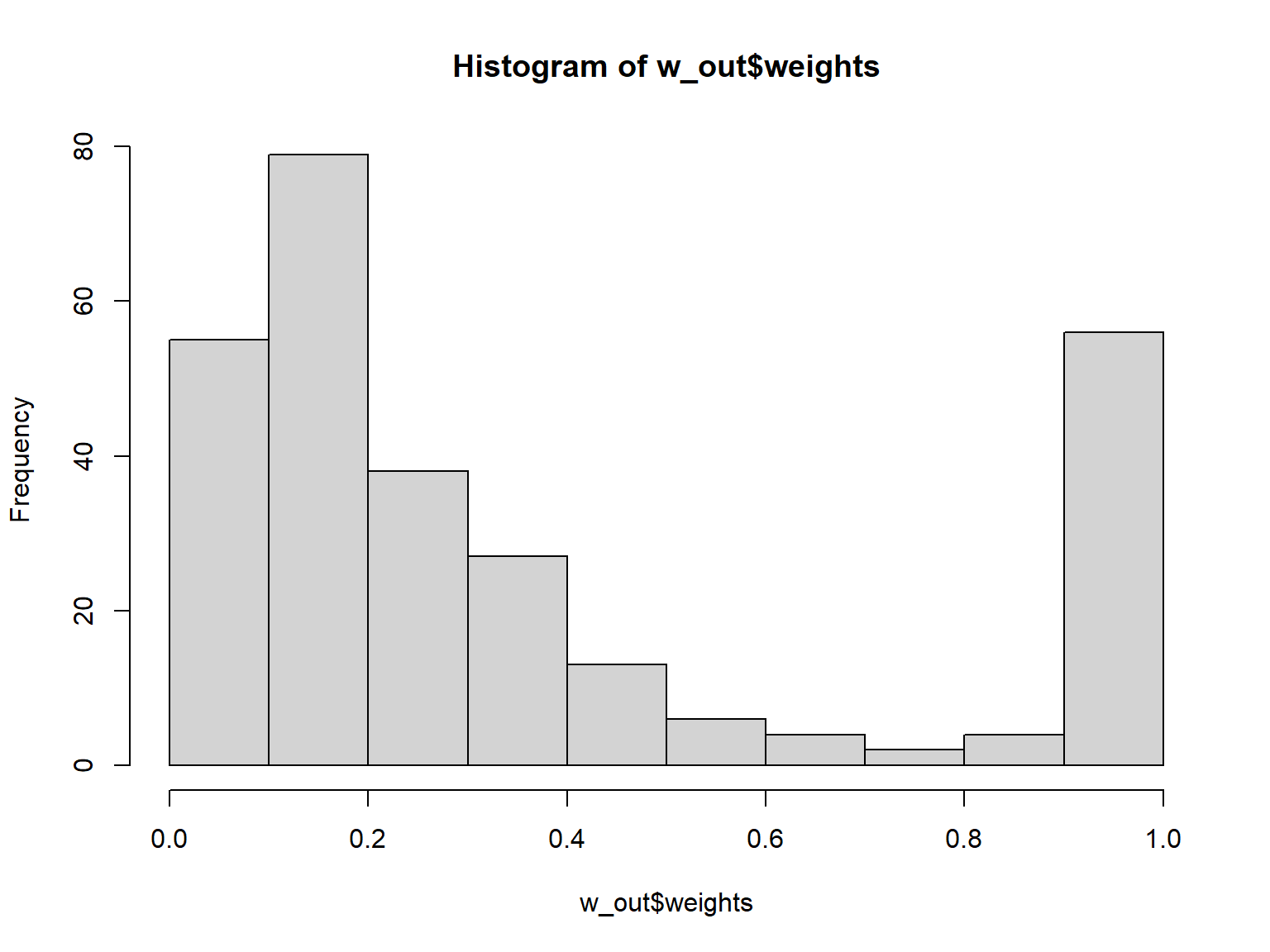

Code

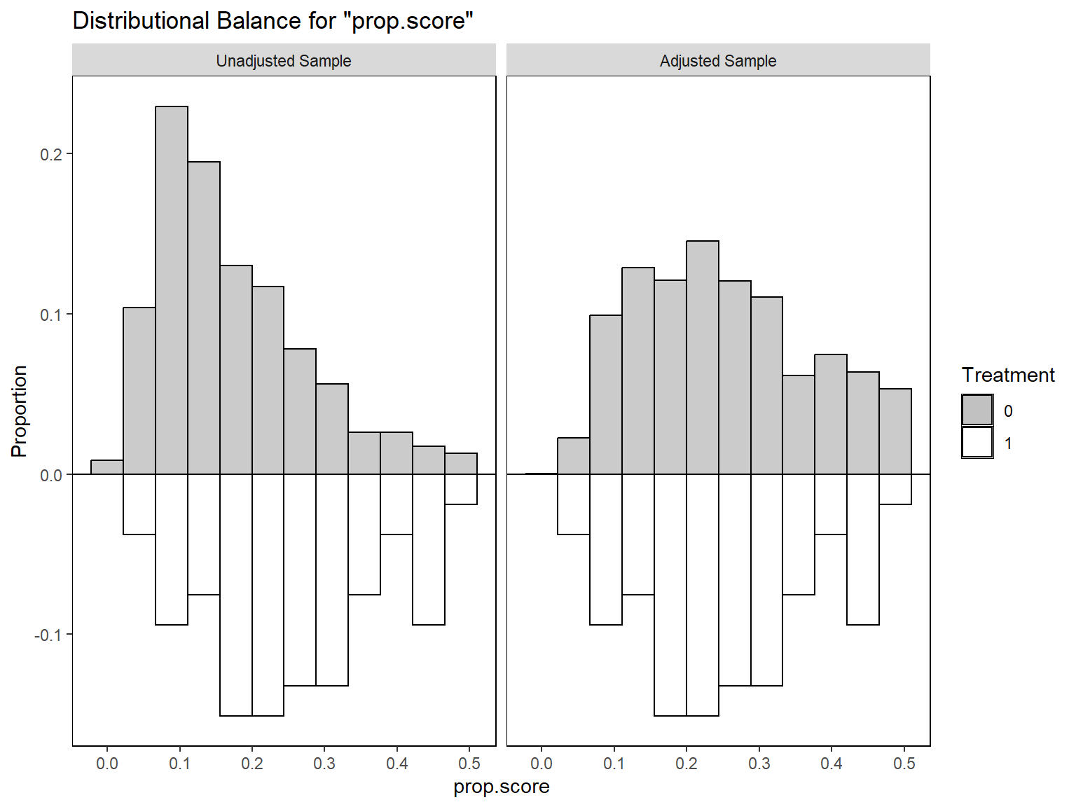
# assess covariate balance
library(cobalt) # https://ngreifer.github.io/cobalt/
bal.tab(w_out, stats = c("m", "v"), thresholds = c(m = .05))

Balance Measures
                          Type Diff.Adj     M.Threshold V.Ratio.Adj
prop.score            Distance  -0.0361 Balanced, <0.05      0.8680
streams_pre1           Contin.  -0.0229 Balanced, <0.05      3.3904
streams_pre5           Contin.  -0.0215 Balanced, <0.05      3.4059
streams_pre10          Contin.  -0.0185 Balanced, <0.05      3.2658
danceability           Contin.   0.0358 Balanced, <0.05      1.1257
valence                Contin.  -0.0067 Balanced, <0.05      1.0781
duration_ms            Contin.   0.0211 Balanced, <0.05      0.8281
playlist_follower_pre  Contin.   0.0106 Balanced, <0.05      2.1967
n_playlists_pre        Contin.   0.0186 Balanced, <0.05      1.4048

Balance tally for mean differences
                    count
Balanced, <0.05         9
Not Balanced, >0.05     0

Variable with the greatest mean difference
     Variable Diff.Adj     M.Threshold
 danceability   0.0358 Balanced, <0.05

Effective sample sizes
           Control Treated
Unadjusted   231.       53
Adjusted     140.4      53

Code

bal.plot(w_out,
    var.name = "prop.score", which = "both",
    type = "histogram", mirror = T, colors = c("grey", "white")
)

Code

love.plot(w_out,
    var.order = "unadjusted",
    line = TRUE,
    threshold = .1,
    colors = c("darkgrey", "black")
)

Estimation using weights

The weights calculated in the previous step can be passed to the fixest package.

Code

# extract weights
weight_df <- data.frame(song_id = psm_matching$song_id, weight = w_out$weights)
# merge weights to data
did_data <- plyr::join(did_data, weight_df[, c("song_id", "weight")], type = "left", match = "first")
# estimate weighted DiD model
did_m6 <- feols(
    log(streams + 1) ~ treated * post |
        song_id + week,
    cluster = "song_id",
    weights = did_data[did_data$week != as.Date("2018-03-19"), "weight"],
    data = did_data %>% dplyr::filter(week != as.Date("2018-03-19"))
)
# compare results with non-matched sample
etable(did_m2, did_m6, se = "cluster", headers = c("unweighted", "weighted"))

Synthetic control

Estimation using generalized synthetic controls (gsynth package Xu and Liu 2021)) to ensure similarity between treated and control units.

Code

library(gsynth) # https://yiqingxu.org/packages/gsynth/
# inspect data
panelview(streams ~ treated_post, data = did_data, index = c("song_id", "week"), pre.post = TRUE, by.timing = TRUE)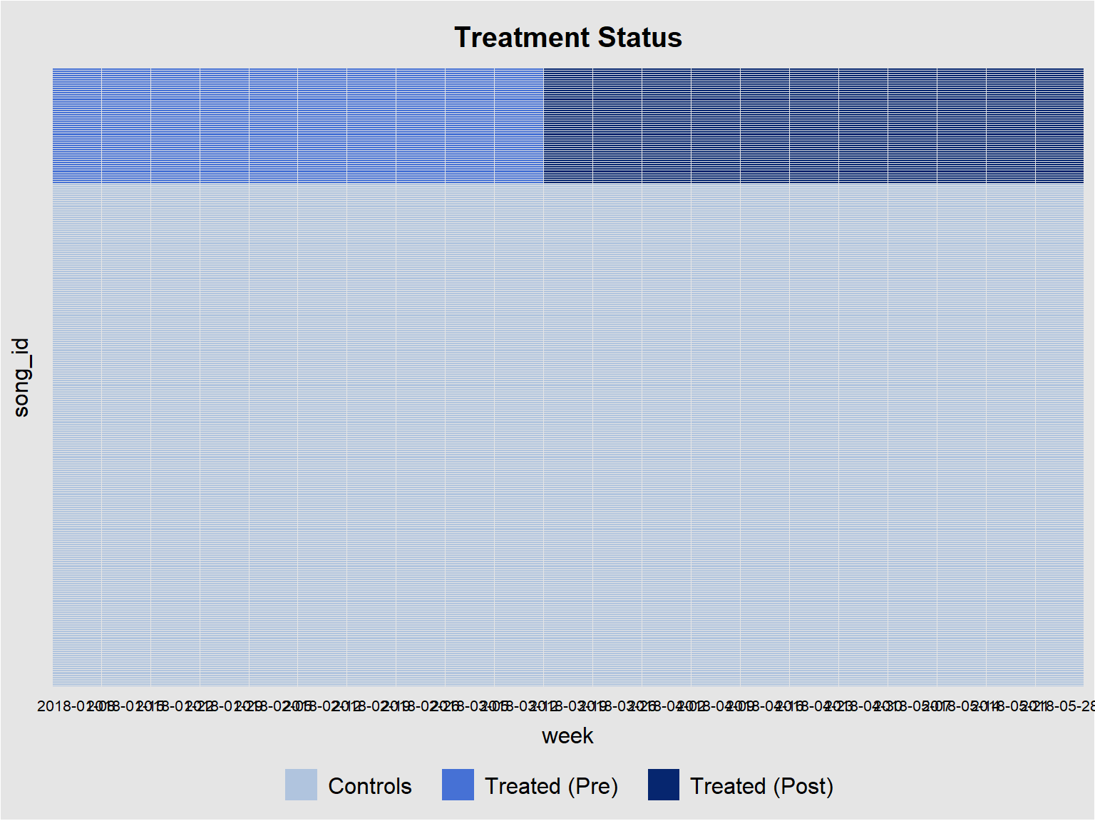

Code

did_data$log_streams <- log(did_data$streams)
did_data$log_ig_followers <- log(did_data$ig_followers + 1)
did_data$log_playlist_followers <- log(did_data$playlist_followers + 1)
did_data$log_n_postings <- log(did_data$n_postings + 1)
did_data$log_n_playlists <- log(did_data$n_playlists + 1)

# estimation
sc_m1 <- gsynth(log_streams ~ treated_post, #+
    # log_ig_followers + log_playlist_followers +
    # log_n_postings + log_n_playlists,
    data = did_data,
    # r = 0, CV = FALSE,
    r = c(0, 5), CV = TRUE,
    index = c("song_id", "week"), force = "two-way", se = TRUE,
    inference = "parametric", nboots = 1000,
    parallel = TRUE, cores = 4
)

Parallel computing ...
Cross-validating ... 
 r = 0; sigma2 = 0.03054; IC = -3.04961; PC = 0.02896; MSPE = 0.01636
 r = 1; sigma2 = 0.01090; IC = -3.64449; PC = 0.01456; MSPE = 0.01314
 r = 2; sigma2 = 0.00728; IC = -3.61560; PC = 0.01255; MSPE = 0.01061*
 r = 3; sigma2 = 0.00542; IC = -3.48293; PC = 0.01144; MSPE = 0.01476
 r = 4; sigma2 = 0.00421; IC = -3.30913; PC = 0.01054; MSPE = 0.02762
 r = 5; sigma2 = 0.00353; IC = -3.06336; PC = 0.01021; MSPE = 0.03692

 r* = 2


Simulating errors ...
Bootstrapping ...

Code

# ATT
cumu_eff <- cumuEff(sc_m1, cumu = TRUE, id = NULL, period = c(0, 10)) # cumulative  ATT
plot(sc_m1) # effects plot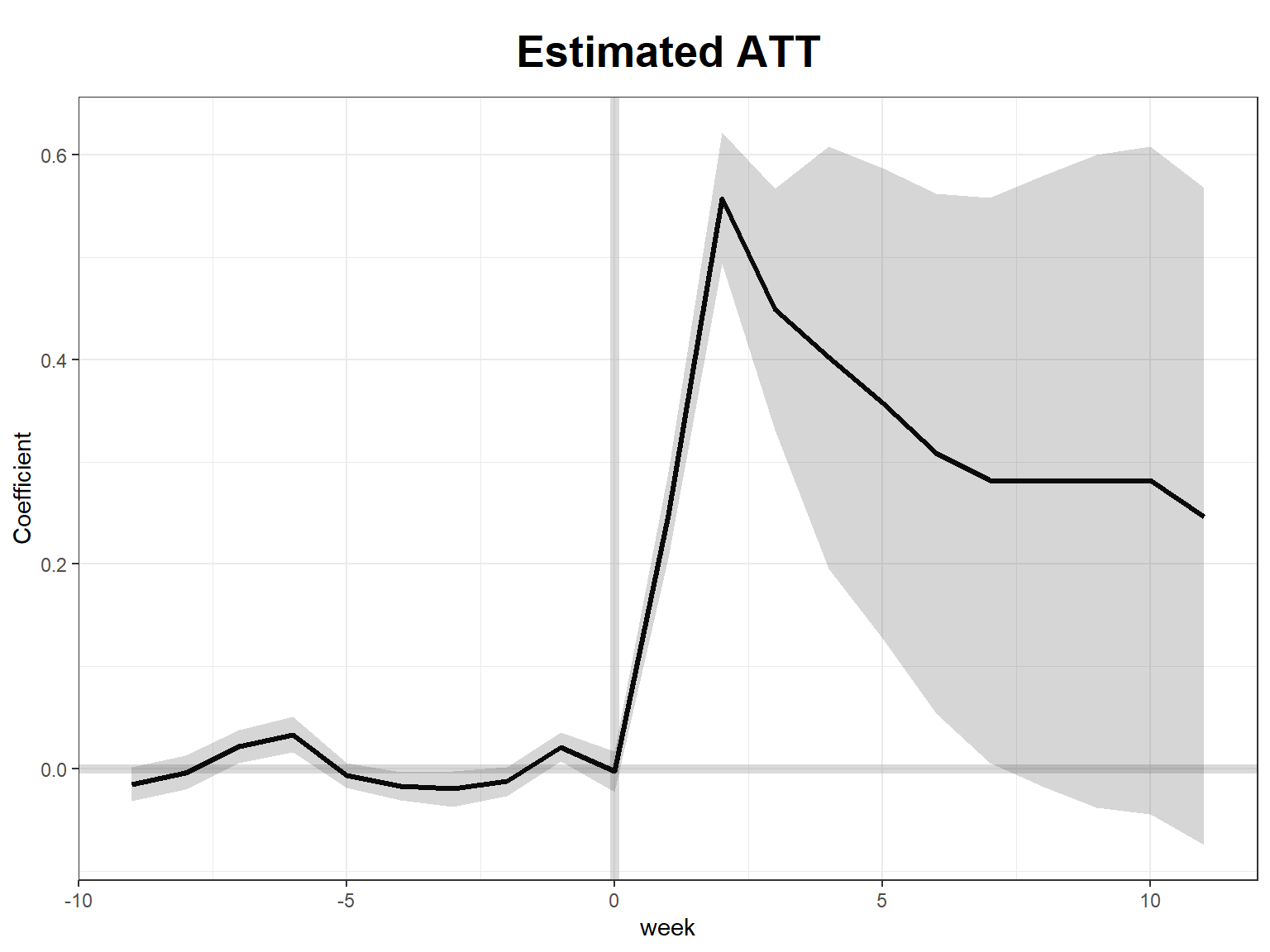

Code

plot(sc_m1, type = "raw") # incl raw data

Code

plot(sc_m1, type = "gap", id = 3, main = "Example song")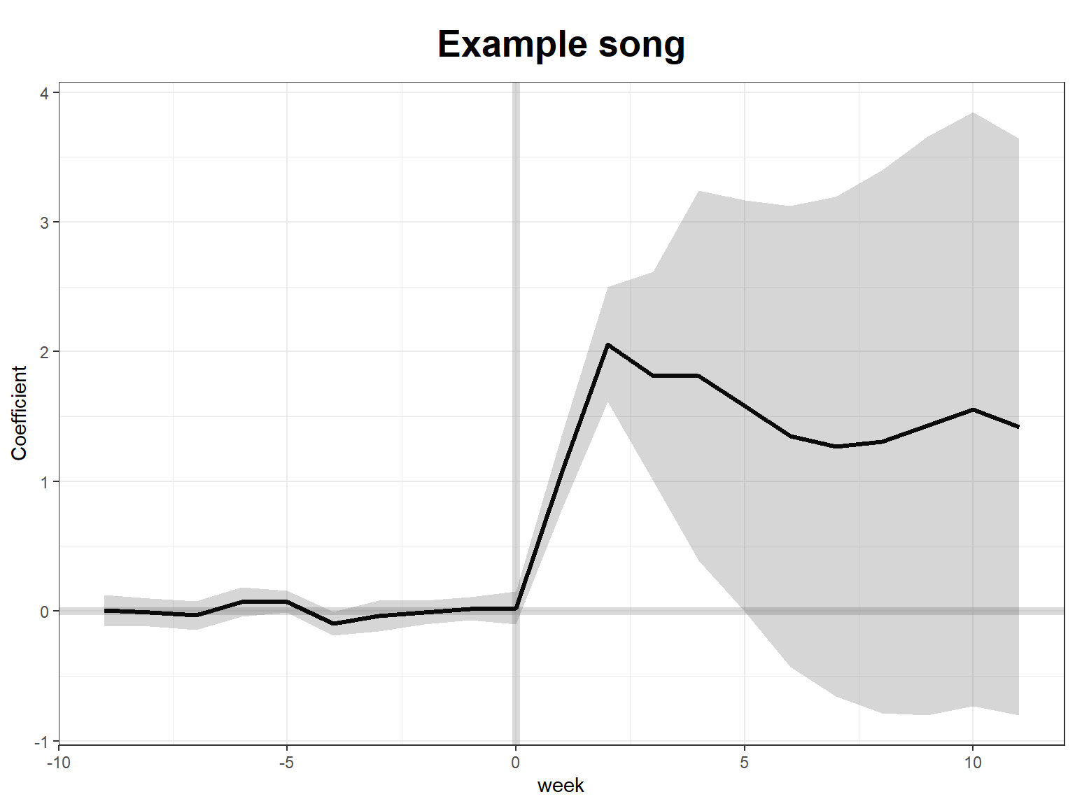

ATT and CI per period:

Code

sc_m1$est.att

            ATT        S.E.     CI.lower      CI.upper              p.value
-9 -0.014939001 0.009835151 -0.034215543  0.0043375411 0.128777691495282509
-8 -0.003669063 0.009118334 -0.021540670  0.0142025425 0.687402103844154233
-7  0.021725473 0.008478780  0.005107370  0.0383435769 0.010397104371477450
-6  0.033490588 0.009877606  0.014130836  0.0528503397 0.000697507019014054
-5 -0.006275912 0.007080434 -0.020153308  0.0076014844 0.375416100662471663
-4 -0.017000624 0.006890679 -0.030506107 -0.0034951408 0.013617757954593745
-3 -0.019701873 0.009574440 -0.038467432 -0.0009363152 0.039613447849829786
-2 -0.012366284 0.007451635 -0.026971220  0.0022386521 0.097007087157054306
-1  0.021280904 0.007589369  0.006406013  0.0361557941 0.005046647266487847
0  -0.002544207 0.009757656 -0.021668862  0.0165804482 0.794293362266164982
1   0.247998960 0.022163285  0.204559719  0.2914382009 0.000000000000000000
2   0.557737597 0.033714332  0.491658720  0.6238164743 0.000000000000000000
3   0.448963532 0.064991561  0.321582413  0.5763446521 0.000000000004914291
4   0.401958108 0.111697584  0.183034865  0.6208813505 0.000319899810204527
5   0.357872236 0.124435205  0.113983717  0.6017607553 0.004027847000901419
6   0.308301033 0.138397423  0.037047068  0.5795549978 0.025903857310217937
7   0.282250622 0.151077118 -0.013855089  0.5783563320 0.061726498538240859
8   0.281267992 0.164722091 -0.041581375  0.6041173577 0.087723497357681257
9   0.281026795 0.178466314 -0.068760753  0.6308143427 0.115331026171494599
10  0.281880510 0.182777276 -0.076356367  0.6401173879 0.123023145010136004
11  0.246654834 0.178396214 -0.102995321  0.5963049895 0.166780277820889333
   n.Treated
-9         0
-8         0
-7         0
-6         0
-5         0
-4         0
-3         0
-2         0
-1         0
0          0
1         53
2         53
3         53
4         53
5         53
6         53
7         53
8         53
9         53
10        53
11        53

ATT

Code

sc_m1$est.avg # ATT

        Estimate      S.E. CI.lower CI.upper     p.value
ATT.avg 0.335992 0.1190547 0.102649 0.569335 0.004770071

\(\beta\) coefficients from factor model

Code

sc_m1$est.beta # beta coefficients from factor model

NULL

Counterfactual prediction

Code

# counterfactual prediction
plot(sc_m1, type = "counterfactual", raw = "none", xlab = "Time")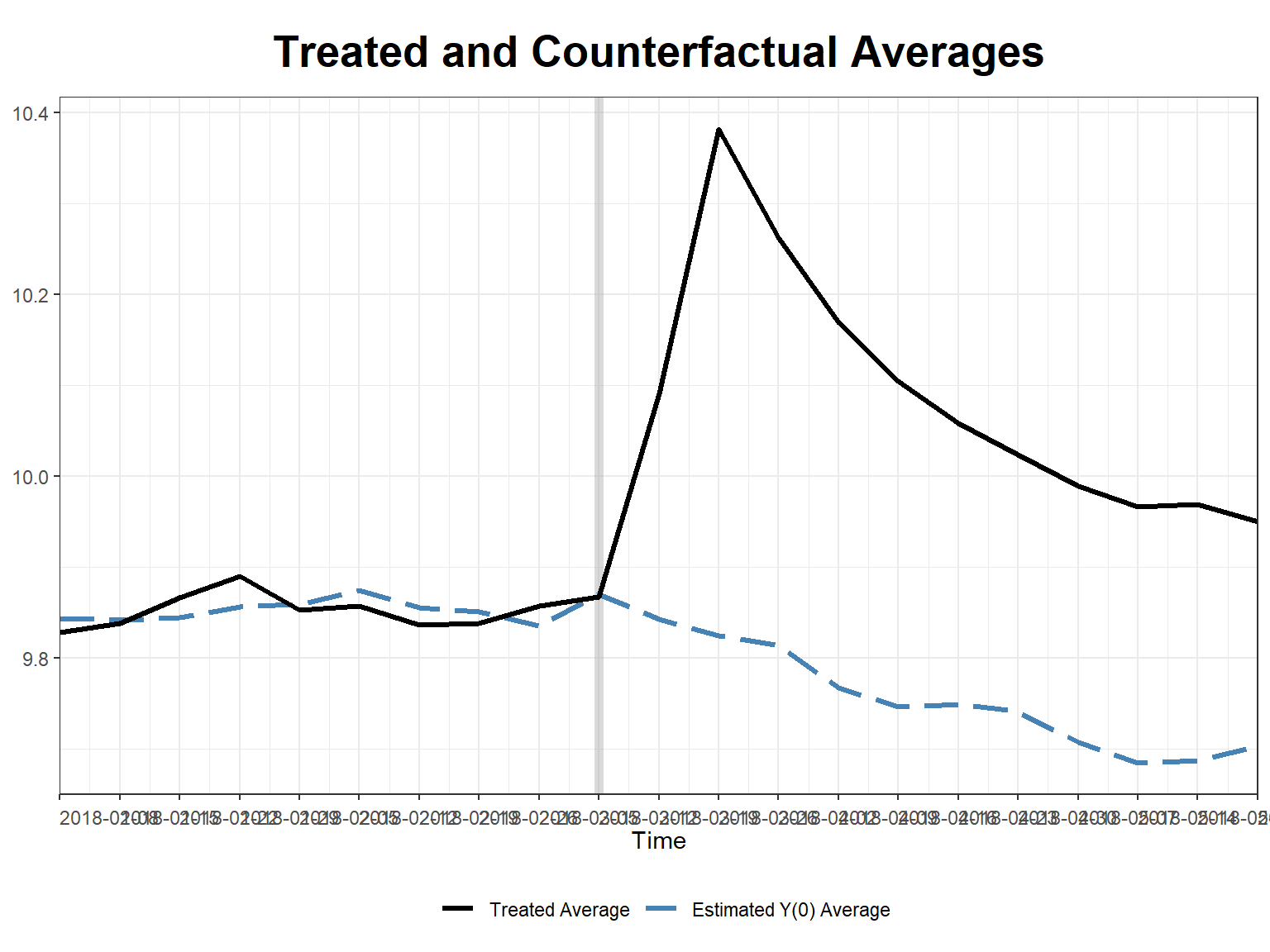

Code

plot(sc_m1, type = "counterfactual", raw = "all") # incl raw data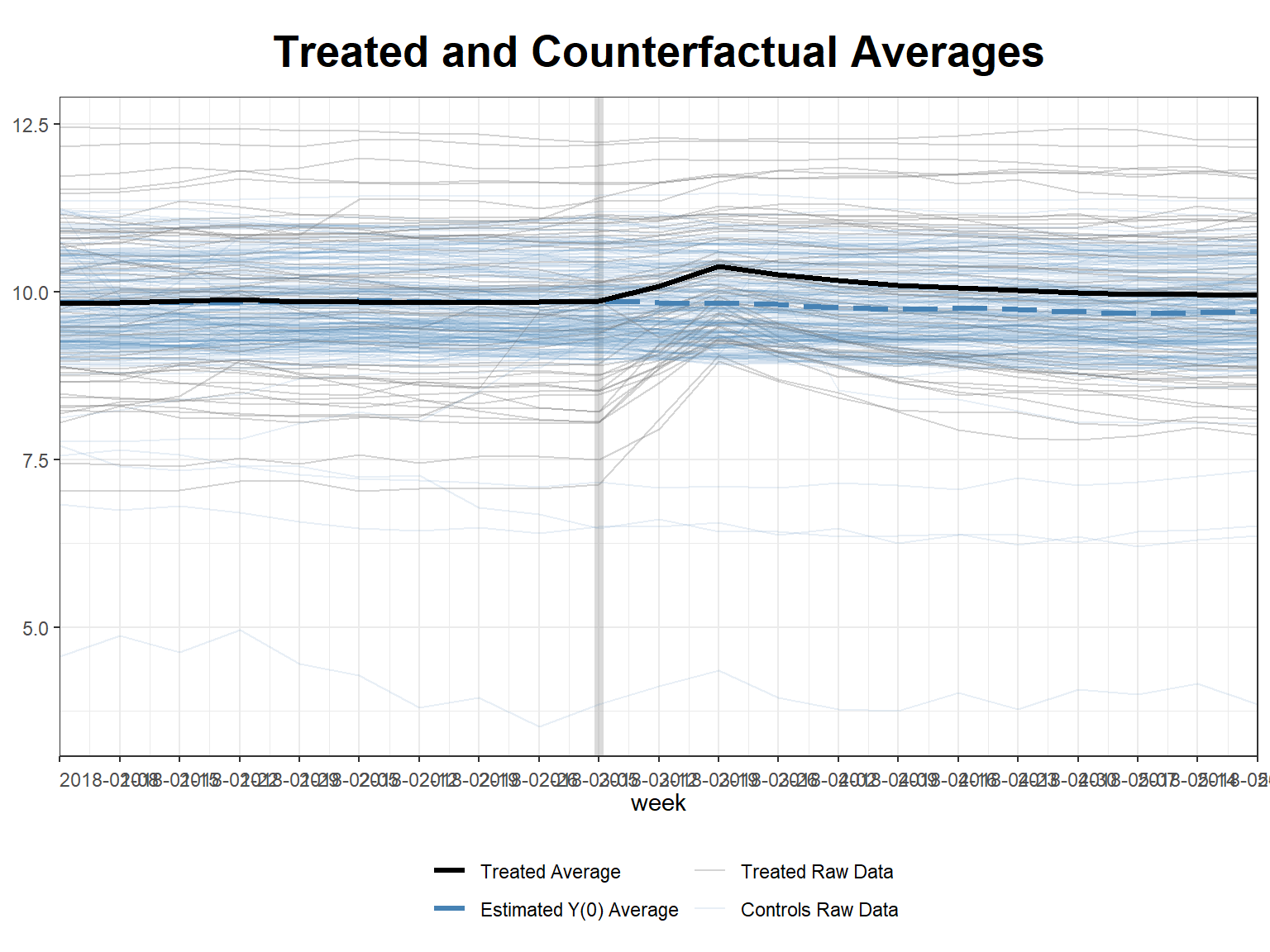

Code

plot(sc_m1, type = "counterfactual", id = 3) # for individual units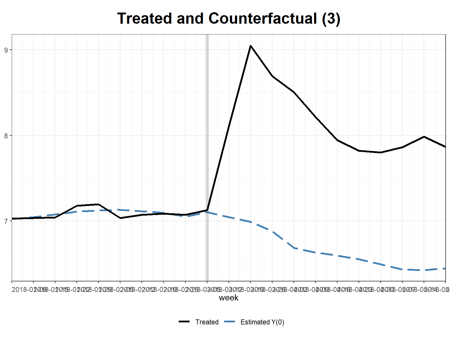

Factor model

Code

# factor model
plot(sc_m1, type = "factors", xlab = "Time")

Code

plot(sc_m1, type = "loadings")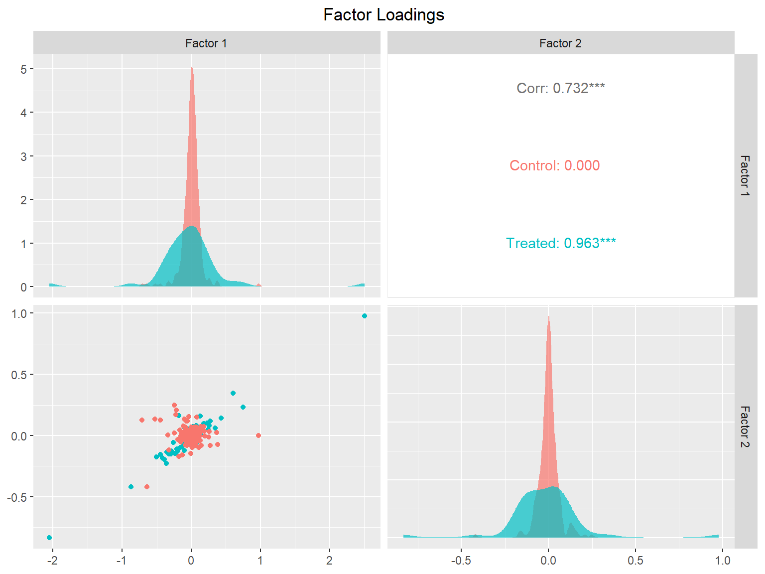

Synthetic Difference-in-Differences

Estimation using synthetic difference-in-differences proposed by Arkhangelsky et al. (2021) and implemented in the synthdid package (Arkhangelsky 2023).

Code

library(synthdid) # https://synth-inference.github.io/synthdid/articles/synthdid.html
# data pre-processing
did_data_synthdid <- did_data %>%
    dplyr::select(song_id, week, streams, treated_post) %>%
    dplyr::mutate(streams = log(streams)) %>%
    as.data.frame()
# data setup
setup <- panel.matrices(did_data_synthdid)
# estimation
synthdid_m1 <- synthdid_estimate(setup$Y, setup$N0, setup$T0)

Code

# treatment effect
plot(synthdid_m1)

Code

se <- sqrt(vcov(synthdid_m1, method = "placebo"))
sprintf("point estimate: %1.2f", synthdid_m1)

[1] "point estimate: 0.27"

Code

sprintf("95%% CI (%1.2f, %1.2f)", synthdid_m1 - 1.96 * se, synthdid_m1 + 1.96 * se)

[1] "95% CI (0.21, 0.32)"

Visualizing the results

Code

# control unit contribution
synthdid_units_plot(synthdid_m1, se.method = "placebo")

Code

# assessing parallel pre-treatment trends
plot(synthdid_m1, overlay = 1, se.method = "placebo")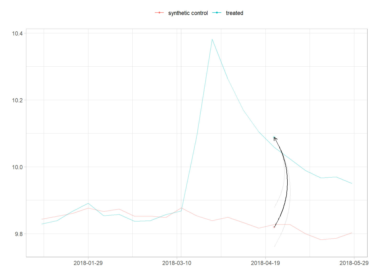

Code

plot(synthdid_m1, overlay = .8, se.method = "placebo")

Code

# compare to standard DiD estimator and synthetic control
synthdid_m2 <- did_estimate(setup$Y, setup$N0, setup$T0)
synthdid_m3 <- sc_estimate(setup$Y, setup$N0, setup$T0)
estimates <- list(synthdid_m2, synthdid_m1, synthdid_m3)
names(estimates) <- c("Diff-in-Diff", "Synthetic Diff-in-Diff", "Synthetic Control")
print(unlist(estimates))

          Diff-in-Diff Synthetic Diff-in-Diff      Synthetic Control 
             0.2836426              0.2683169              0.2908847 

Time-varying treatment effects

Staggered adoption

Visualization of the panel structure using panelView.

Code

# staggered adoption
# https://yiqingxu.org/packages/gsynth/articles/tutorial.html
# upcoming package: https://github.com/zachporreca/staggered_adoption_synthdid
# load data
did_data_staggered <- fread("https://raw.githubusercontent.com/WU-RDS/RMA2022/main/data/did_data_staggered.csv")
did_data_staggered$song_id <- as.character(did_data_staggered$song_id)
did_data_staggered$week <- as.Date(did_data_staggered$week)
# data preparation
did_data_staggered$log_streams <- log(did_data_staggered$streams + 1)
did_data_staggered$log_song_age <- log(did_data_staggered$song_age + 1)
did_data_staggered$log_n_playlists <- log(did_data_staggered$n_playlists + 1)
did_data_staggered$log_playlist_followers <- log(did_data_staggered$playlist_followers + 1)
did_data_staggered$log_n_postings <- log(did_data_staggered$n_postings + 1)

# inspect data
panelview(log_streams ~ treated_post, data = did_data_staggered, index = c("song_id", "week"), pre.post = TRUE, by.timing = TRUE)

Code

panelview(log_streams ~ treated_post, data = did_data_staggered, index = c("song_id", "week"), type = "outcome")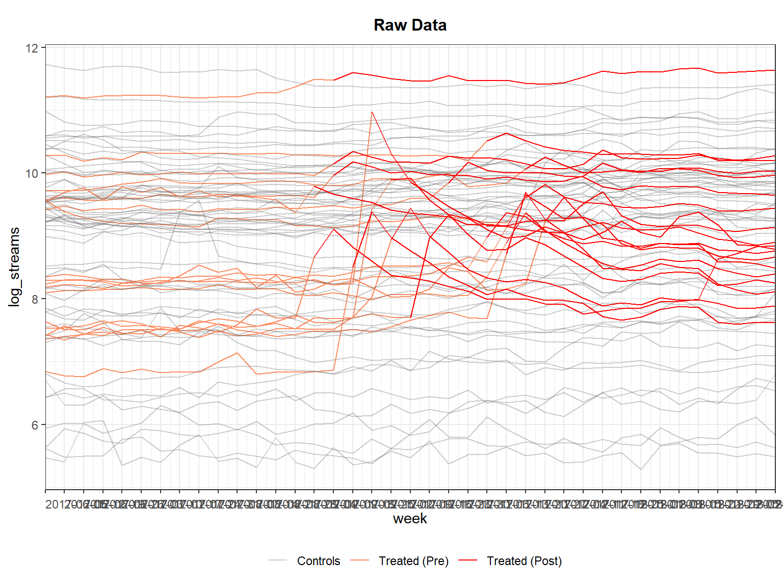

Code

panelview(log_streams ~ treated_post, data = did_data_staggered, index = c("song_id", "week"), type = "outcome", main = "Number of weekly streams", by.group = TRUE)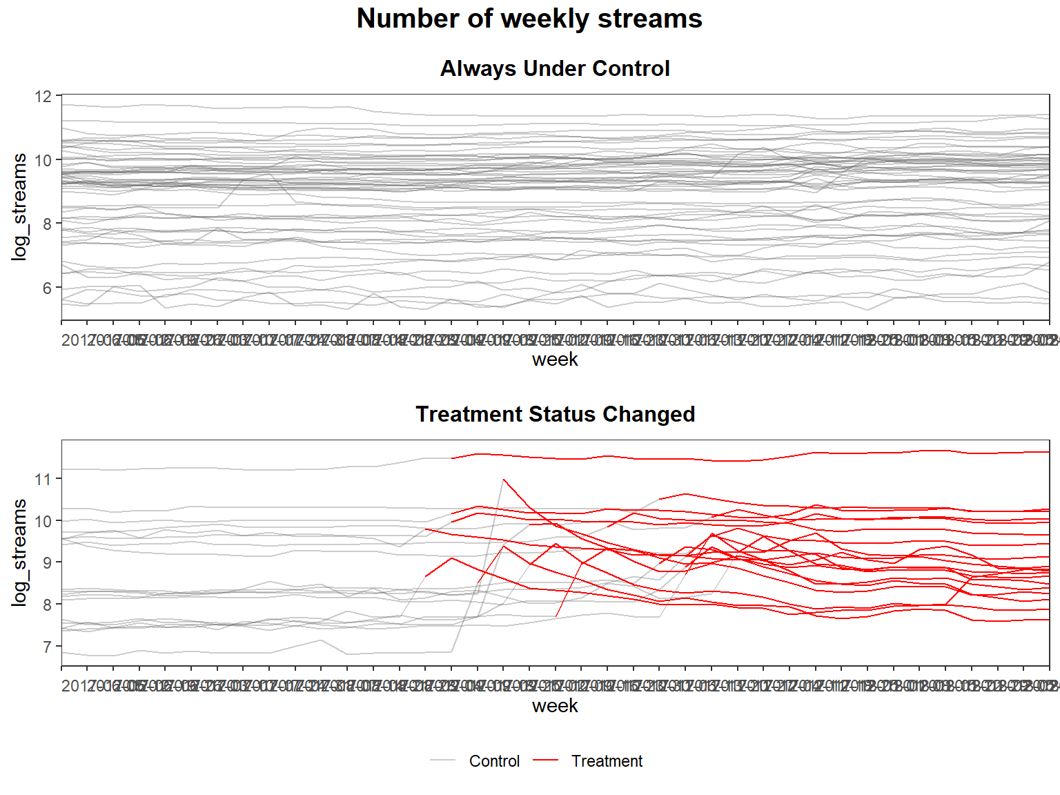

Multiple packages implement estimators appropriate for staggered adoption. Among them are gsynth, did, and fixest (latter not shown here, see ?sunab). There is also forthcoming package to extend synthdid.

Synthetic control

Estimation using gsynth.

Code

# run model
stag_m1 <- gsynth(log_streams ~ treated_post + log_song_age + log_n_playlists + log_playlist_followers + log_n_postings,
    data = did_data_staggered, index = c("song_id", "week"),
    se = TRUE, inference = "parametric",
    r = c(0, 5), CV = TRUE, force = "two-way",
    nboots = 1000, seed = 02139
)

Parallel computing ...
Cross-validating ... 
 r = 0; sigma2 = 0.01479; IC = -3.87432; PC = 0.01414; MSPE = 0.01824
 r = 1; sigma2 = 0.00835; IC = -4.12631; PC = 0.00939; MSPE = 0.01593*
 r = 2; sigma2 = 0.00721; IC = -3.96033; PC = 0.00933; MSPE = 0.01658
 r = 3; sigma2 = 0.00632; IC = -3.78512; PC = 0.00927; MSPE = 0.01738
 r = 4; sigma2 = 0.00543; IC = -3.63799; PC = 0.00889; MSPE = 0.01850
 r = 5; sigma2 = 0.00476; IC = -3.47679; PC = 0.00862; MSPE = 0.01968

 r* = 1


Simulating errors ...
Bootstrapping ...

Code

# ATT
cumu_eff <- cumuEff(stag_m1, cumu = TRUE, id = NULL, period = c(0, 10)) # cumulative  ATT
cumu_eff

$catt
 [1] 0.07190787 0.72201771 1.71260141 2.48563521 3.05755892 3.51060998
 [7] 3.84717027 4.13102323 4.37933938 4.59954027 4.74789137

$est.catt
         CATT       S.E.   CI.lower  CI.upper p.value
0  0.07190787 0.02003151 0.03992271 0.1194863       0
1  0.72201771 0.04301672 0.65409399 0.8208971       0
2  1.71260141 0.06983871 1.59990247 1.8725702       0
3  2.48563521 0.10200752 2.31775373 2.7213509       0
4  3.05755892 0.13773130 2.82256342 3.3661126       0
5  3.51060998 0.17779308 3.20168824 3.9084697       0
6  3.84717027 0.22184775 3.47242065 4.3324431       0
7  4.13102323 0.26962386 3.65590487 4.7219944       0
8  4.37933938 0.31951904 3.81504646 5.0588090       0
9  4.59954027 0.37444657 3.92248425 5.4222747       0
10 4.74789137 0.43547676 3.96206121 5.6938628       0

Code

plot(stag_m1) # effects plot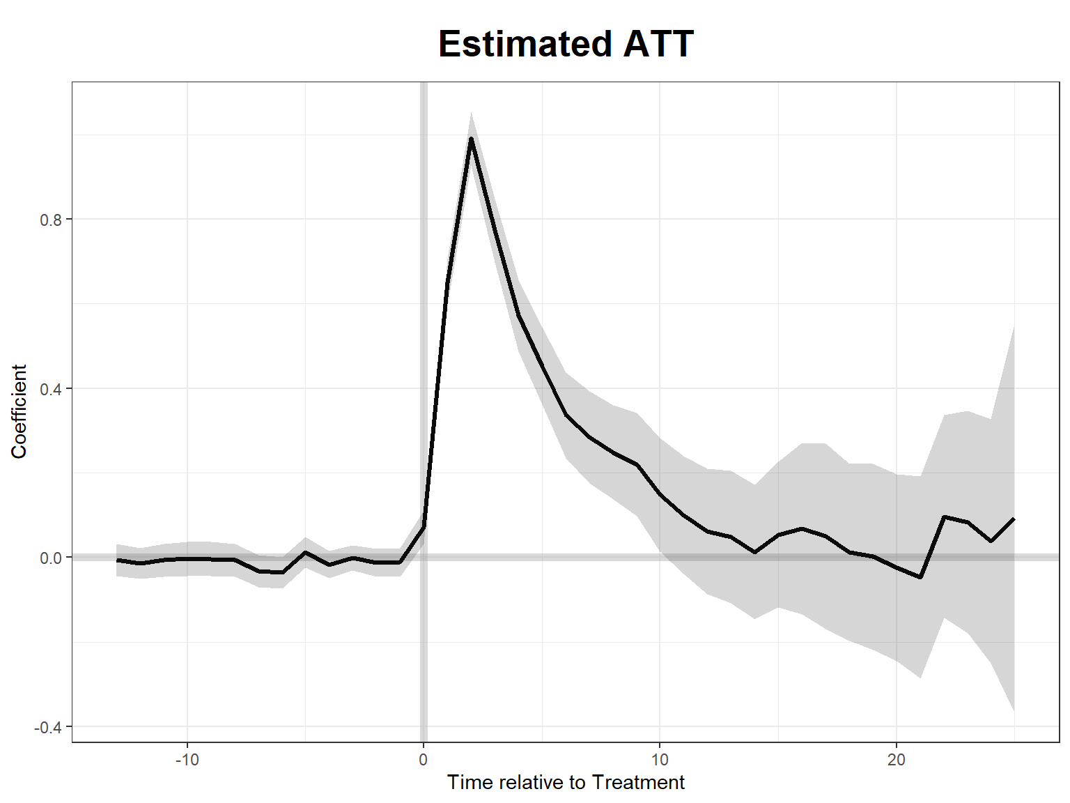

Code

plot(stag_m1, type = "gap")

Code

plot(stag_m1, type = "gap", id = 79, main = "Example song")

ATT and CI per period

Code

stag_m1$est.att # ATT and CI per period

              ATT       S.E.    CI.lower    CI.upper             p.value
-13 -0.0054054341 0.01927440 -0.04318256 0.032371694 0.77913511178311090
-12 -0.0138774521 0.01843034 -0.05000025 0.022245344 0.45146919840641608
-11 -0.0067336063 0.01962561 -0.04519909 0.031731877 0.73152091468251035
-10 -0.0033576945 0.02059757 -0.04372818 0.037012796 0.87050731178397744
-9  -0.0036965022 0.02036289 -0.04360704 0.036214032 0.85595056429849214
-8  -0.0065909945 0.01965459 -0.04511328 0.031931291 0.73736766963486344
-7  -0.0323289393 0.01939282 -0.07033817 0.005680290 0.09550304970414913
-6  -0.0364515566 0.01912374 -0.07393340 0.001030286 0.05663862295093280
-5   0.0123884296 0.01872200 -0.02430603 0.049082885 0.50816079660724012
-4  -0.0172533778 0.01650275 -0.04959817 0.015091417 0.29579884548013347
-3  -0.0004454345 0.01508285 -0.03000727 0.029116401 0.97643988147333327
-2  -0.0124497951 0.01690927 -0.04559135 0.020691756 0.46156603216607728
-1  -0.0115372520 0.01698733 -0.04483181 0.021757302 0.49703137286526688
0    0.0719078706 0.02003151  0.03264683 0.111168909 0.00033101069001717
1    0.6501098402 0.02864717  0.59396242 0.706257261 0.00000000000000000
2    0.9905837035 0.03208610  0.92769610 1.053471311 0.00000000000000000
3    0.7730337980 0.03857064  0.69743674 0.848630859 0.00000000000000000
4    0.5719237115 0.04324208  0.48717080 0.656676628 0.00000000000000000
5    0.4530510576 0.04702741  0.36087904 0.545223080 0.00000000000000000
6    0.3365602893 0.05174525  0.23514146 0.437979121 0.00000000007811973
7    0.2838529600 0.05565152  0.17477798 0.392927942 0.00000033868137450
8    0.2483161483 0.05662558  0.13733204 0.359300254 0.00001158638863741
9    0.2202008899 0.06236095  0.09797568 0.342426104 0.00041388184796221
10   0.1483510977 0.06859961  0.01389834 0.282803857 0.03057466523178398
11   0.0996620908 0.07098555 -0.03946702 0.238791206 0.16032563330680683
12   0.0617311668 0.07592444 -0.08707801 0.210540339 0.41618335658991956
13   0.0485301714 0.07982027 -0.10791467 0.204975017 0.54319204471373106
14   0.0126136638 0.08103570 -0.14621339 0.171440722 0.87630446794065309
15   0.0538661163 0.08791188 -0.11843800 0.226170236 0.54005586340453293
16   0.0677489377 0.10328158 -0.13467924 0.270177113 0.51184766163355100
17   0.0496789910 0.11183431 -0.16951223 0.268870209 0.65688382980198634
18   0.0116951540 0.10677328 -0.19757662 0.220966930 0.91278007049659315
19   0.0014565251 0.11210216 -0.21825967 0.221172722 0.98963350751376122
20  -0.0236014674 0.11277651 -0.24463936 0.197436427 0.83423243404798764
21  -0.0479777209 0.12199573 -0.28708496 0.191129521 0.69411729322338056
22   0.0967723399 0.12262157 -0.14356153 0.337106208 0.42999800925794518
23   0.0836290245 0.13418156 -0.17936199 0.346620044 0.53311844165248390
24   0.0385864510 0.14700569 -0.24953941 0.326712314 0.79294932185020772
25   0.0928196596 0.23493023 -0.36763513 0.553274452 0.69277309336814086
    n.Treated
-13         0
-12         0
-11         0
-10         0
-9          0
-8          0
-7          0
-6          0
-5          0
-4          0
-3          0
-2          0
-1          0
0           0
1          19
2          19
3          19
4          19
5          19
6          19
7          19
8          19
9          19
10         19
11         19
12         19
13         19
14         18
15         16
16         13
17         11
18         11
19         10
20         10
21          9
22          7
23          6
24          5
25          2

ATT

Code

stag_m1$est.avg # ATT

         Estimate       S.E. CI.lower  CI.upper       p.value
ATT.avg 0.2640589 0.06225465 0.142042 0.3860758 0.00002219394

\(\beta\) from factor model

Code

stag_m1$est.beta # beta coefficients form factor model

                              beta        S.E.     CI.lower    CI.upper
log_song_age           -1.13361285 0.418112413 -1.953098123 -0.31412758
log_n_playlists        -0.04535966 0.069146370 -0.180884054  0.09016474
log_playlist_followers  0.09602444 0.019785461  0.057245652  0.13480323
log_n_postings          0.01396278 0.005562191  0.003061087  0.02486448
                              p.value
log_song_age           0.006702737142
log_n_playlists        0.511827471407
log_playlist_followers 0.000001214342
log_n_postings         0.012062783443

counterfactual prediction

Code

plot(stag_m1, type = "raw")

Code

plot(stag_m1, type = "counterfactual", id = 79) # for individual units

factor model

Code

plot(stag_m1, type = "factors", xlab = "Time")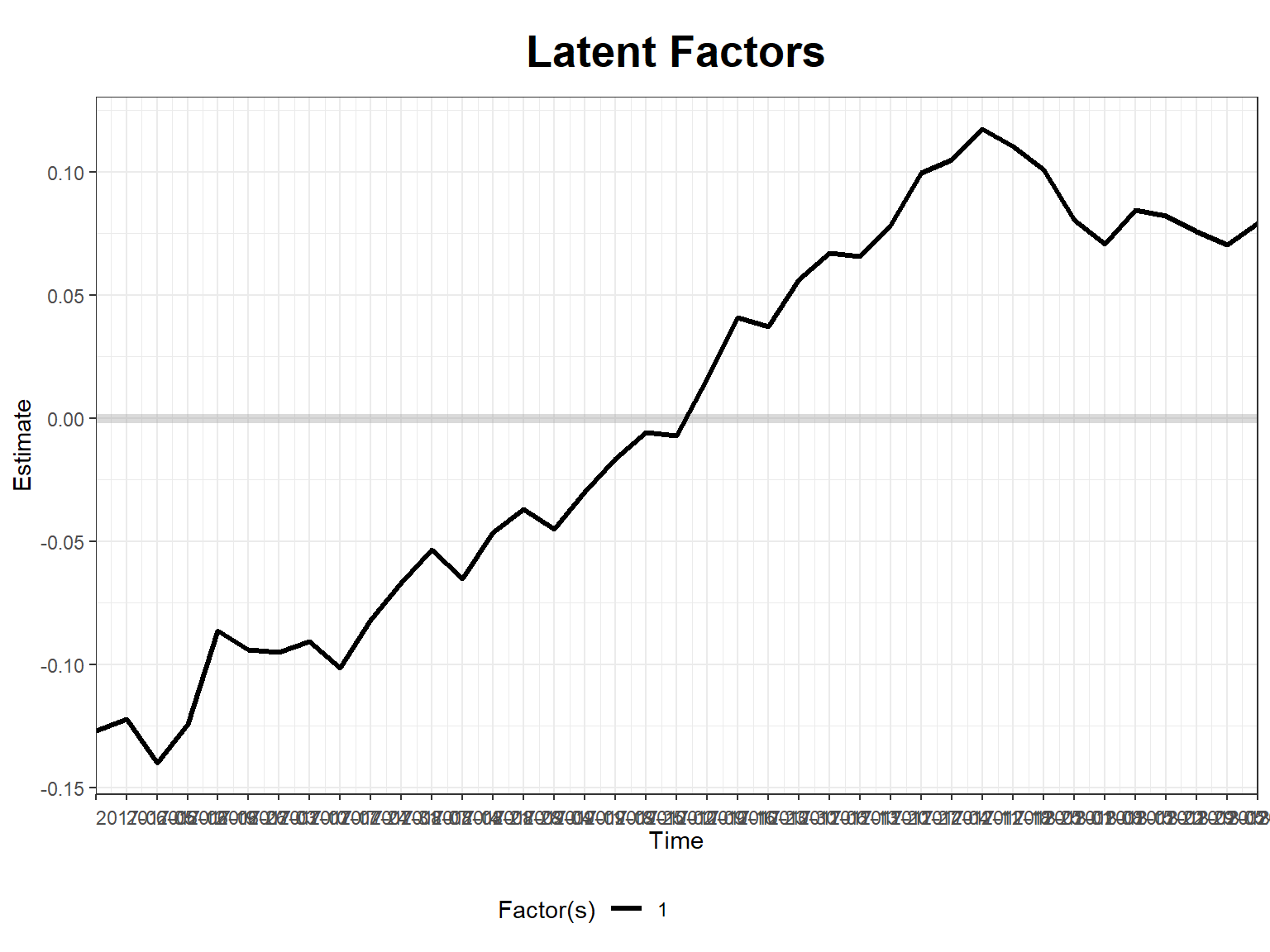

Code

plot(stag_m1, type = "loadings")

Loadings for the first factor are shown...

Staggered Difference-in-Differences

Estimation using did.

Code

# staggered did
did_data_staggered$period <- as.numeric(factor(as.character(did_data_staggered$week),
    levels = as.character(sort(unique(did_data_staggered$week)))
))
# add first period treated
did_data_staggered_G <- did_data_staggered |>
    filter(treated == 1, week == treat_week) |>
    select(song_id, G = period)
did_data_staggered <- left_join(did_data_staggered,
    did_data_staggered_G,
    by = "song_id"
)
did_data_staggered$G <- coalesce(did_data_staggered$G, 0)
did_data_staggered$id <- as.numeric(did_data_staggered$song_id)

set.seed(123)
# increase bootstrap for reliability!
did_stag <- att_gt(
    yname = "log_streams",
    tname = "period",
    idname = "id",
    gname = "G",
    biters = 2000,
    data = did_data_staggered
)

Overall ATT

Code

## Full aggregation
aggte(did_stag, type = "simple", biters = 20000)

Call:
aggte(MP = did_stag, type = "simple", biters = 20000)

Reference: Callaway, Brantly and Pedro H.C. Sant'Anna.  "Difference-in-Differences with Multiple Time Periods." Journal of Econometrics, Vol. 225, No. 2, pp. 200-230, 2021. <https://doi.org/10.1016/j.jeconom.2020.12.001>, <https://arxiv.org/abs/1803.09015> 

    ATT    Std. Error     [ 95%  Conf. Int.]  
 0.3398        0.0984      0.147      0.5327 *


---
Signif. codes: `*' confidence band does not cover 0

Control Group:  Never Treated,  Anticipation Periods:  0
Estimation Method:  Doubly Robust

ATT by time relative to treatment

Code

## Aggregate time relative to treatment
aggte(did_stag, type = "dynamic")

Call:
aggte(MP = did_stag, type = "dynamic")

Reference: Callaway, Brantly and Pedro H.C. Sant'Anna.  "Difference-in-Differences with Multiple Time Periods." Journal of Econometrics, Vol. 225, No. 2, pp. 200-230, 2021. <https://doi.org/10.1016/j.jeconom.2020.12.001>, <https://arxiv.org/abs/1803.09015> 


Overall summary of ATT's based on event-study/dynamic aggregation:  
   ATT    Std. Error     [ 95%  Conf. Int.]  
 0.302        0.1066     0.0931      0.5108 *


Dynamic Effects:
 Event time Estimate Std. Error [95% Simult.  Conf. Band]  
        -25   0.0447     0.0138        0.0087      0.0806 *
        -24  -0.0596     0.0563       -0.2063      0.0871  
        -23  -0.0235     0.0311       -0.1046      0.0577  
        -22   0.0102     0.0155       -0.0302      0.0507  
        -21  -0.0027     0.0214       -0.0584      0.0530  
        -20   0.0107     0.0149       -0.0280      0.0494  
        -19   0.0067     0.0207       -0.0472      0.0606  
        -18   0.0177     0.0260       -0.0499      0.0853  
        -17   0.0158     0.0197       -0.0356      0.0672  
        -16   0.0330     0.0188       -0.0160      0.0820  
        -15  -0.0272     0.0279       -0.0999      0.0455  
        -14   0.0104     0.0177       -0.0357      0.0564  
        -13  -0.0056     0.0208       -0.0597      0.0484  
        -12   0.0108     0.0131       -0.0234      0.0450  
        -11   0.0134     0.0196       -0.0377      0.0645  
        -10  -0.0019     0.0183       -0.0495      0.0457  
         -9   0.0080     0.0162       -0.0343      0.0502  
         -8  -0.0140     0.0171       -0.0586      0.0306  
         -7   0.0115     0.0178       -0.0347      0.0578  
         -6   0.0445     0.0130        0.0106      0.0785 *
         -5  -0.0104     0.0320       -0.0937      0.0729  
         -4   0.0274     0.0133       -0.0073      0.0621  
         -3  -0.0060     0.0287       -0.0807      0.0686  
         -2   0.0132     0.0200       -0.0388      0.0652  
         -1   0.0978     0.1262       -0.2311      0.4267  
          0   0.6528     0.1585        0.2398      1.0658 *
          1   0.9906     0.1564        0.5832      1.3981 *
          2   0.7880     0.1351        0.4359      1.1400 *
          3   0.6068     0.1182        0.2990      0.9147 *
          4   0.4940     0.1085        0.2113      0.7767 *
          5   0.3945     0.1036        0.1245      0.6645 *
          6   0.3554     0.1079        0.0744      0.6365 *
          7   0.3201     0.0937        0.0759      0.5643 *
          8   0.2988     0.0923        0.0584      0.5391 *
          9   0.2358     0.0823        0.0215      0.4501 *
         10   0.1941     0.0879       -0.0349      0.4230  
         11   0.1692     0.0831       -0.0474      0.3857  
         12   0.1531     0.0769       -0.0473      0.3535  
         13   0.1209     0.0795       -0.0861      0.3280  
         14   0.1503     0.0843       -0.0693      0.3698  
         15   0.1738     0.0902       -0.0611      0.4087  
         16   0.1603     0.1078       -0.1206      0.4411  
         17   0.1181     0.1189       -0.1917      0.4280  
         18   0.1067     0.1453       -0.2718      0.4851  
         19   0.0772     0.1385       -0.2836      0.4379  
         20   0.0131     0.1459       -0.3670      0.3932  
         21   0.2654     0.1570       -0.1436      0.6744  
         22   0.2341     0.1805       -0.2362      0.7044  
         23   0.1844     0.2153       -0.3766      0.7455  
         24   0.2925     0.5287       -1.0848      1.6698  
---
Signif. codes: `*' confidence band does not cover 0

Control Group:  Never Treated,  Anticipation Periods:  0
Estimation Method:  Doubly Robust

Code

ggdid(aggte(did_stag, type = "dynamic", biters = 20000))

ATT by treatment time

Code

## Aggregate total effect by treatment time
aggte(did_stag, type = "group", biters = 20000)

Call:
aggte(MP = did_stag, type = "group", biters = 20000)

Reference: Callaway, Brantly and Pedro H.C. Sant'Anna.  "Difference-in-Differences with Multiple Time Periods." Journal of Econometrics, Vol. 225, No. 2, pp. 200-230, 2021. <https://doi.org/10.1016/j.jeconom.2020.12.001>, <https://arxiv.org/abs/1803.09015> 


Overall summary of ATT's based on group/cohort aggregation:  
    ATT    Std. Error     [ 95%  Conf. Int.]  
 0.3485        0.1008      0.151      0.5461 *


Group Effects:
 Group Estimate Std. Error [95% Simult.  Conf. Band]  
    15   0.1647     0.2390       -1.1764      1.5058  
    16   0.1304     0.0839       -0.3406      0.6014  
    17   1.1247     0.0169        1.0298      1.2197 *
    18   0.9600     0.0164        0.8677      1.0523 *
    19  -0.0924     0.1695       -1.0437      0.8589  
    20   0.7733     0.0146        0.6915      0.8551 *
    22   0.1957     0.0167        0.1021      0.2893 *
    24   0.2251     0.1168       -0.4305      0.8808  
    25   0.5162     0.1848       -0.5208      1.5533  
    26   0.2228     0.0411       -0.0081      0.4537  
    27   0.5879     0.0128        0.5161      0.6597 *
---
Signif. codes: `*' confidence band does not cover 0

Control Group:  Never Treated,  Anticipation Periods:  0
Estimation Method:  Doubly Robust

ATT by calendar time

Code

## Aggregate total effect by calendar time
aggte(did_stag, type = "calendar", biters = 20000)

Call:
aggte(MP = did_stag, type = "calendar", biters = 20000)

Reference: Callaway, Brantly and Pedro H.C. Sant'Anna.  "Difference-in-Differences with Multiple Time Periods." Journal of Econometrics, Vol. 225, No. 2, pp. 200-230, 2021. <https://doi.org/10.1016/j.jeconom.2020.12.001>, <https://arxiv.org/abs/1803.09015> 


Overall summary of ATT's based on calendar time aggregation:  
    ATT    Std. Error     [ 95%  Conf. Int.]  
 0.4059        0.1131     0.1842      0.6276 *


Time Effects:
 Time Estimate Std. Error [95% Simult.  Conf. Band]  
   15   0.7019     0.2122        0.1855      1.2182 *
   16   0.4404     0.2917       -0.2694      1.1502  
   17   0.6635     0.2462        0.0644      1.2626 *
   18   1.0019     0.4035        0.0200      1.9839 *
   19   0.7178     0.2658        0.0710      1.3646 *
   20   0.6379     0.2266        0.0863      1.1894 *
   21   0.6142     0.2027        0.1210      1.1074 *
   22   0.5491     0.1880        0.0915      1.0067 *
   23   0.4428     0.1683        0.0333      0.8524 *
   24   0.3142     0.1305       -0.0035      0.6319  
   25   0.4065     0.1231        0.1070      0.7061 *
   26   0.5311     0.1496        0.1672      0.8951 *
   27   0.4944     0.1190        0.2048      0.7841 *
   28   0.4084     0.1183        0.1205      0.6963 *
   29   0.3343     0.1018        0.0866      0.5821 *
   30   0.2937     0.0841        0.0889      0.4984 *
   31   0.2352     0.0751        0.0523      0.4180 *
   32   0.1715     0.0794       -0.0216      0.3646  
   33   0.2120     0.0878       -0.0018      0.4258  
   34   0.2202     0.0795        0.0268      0.4136 *
   35   0.2185     0.0765        0.0325      0.4046 *
   36   0.1657     0.0757       -0.0184      0.3499  
   37   0.1462     0.0856       -0.0621      0.3545  
   38   0.1128     0.0901       -0.1066      0.3322  
   39   0.1131     0.0924       -0.1118      0.3380  
---
Signif. codes: `*' confidence band does not cover 0

Control Group:  Never Treated,  Anticipation Periods:  0
Estimation Method:  Doubly Robust

Comparison to two-way Fixed Effects

The TWFE estimator overestimates the treatment effect in this case

Code

# compare with standard DiD
stag_m2 <- feols(
    log(streams + 1) ~ treated_post |
        song_id + week,
    cluster = "song_id",
    data = did_data_staggered
)
etable(stag_m2, se = "cluster")

Compared to Callaway and Sant’Anna (2021b):

Code

aggte(did_stag, type = "simple", biters = 20000)

Call:
aggte(MP = did_stag, type = "simple", biters = 20000)

Reference: Callaway, Brantly and Pedro H.C. Sant'Anna.  "Difference-in-Differences with Multiple Time Periods." Journal of Econometrics, Vol. 225, No. 2, pp. 200-230, 2021. <https://doi.org/10.1016/j.jeconom.2020.12.001>, <https://arxiv.org/abs/1803.09015> 

    ATT    Std. Error     [ 95%  Conf. Int.]  
 0.3398         0.097     0.1497      0.5299 *


---
Signif. codes: `*' confidence band does not cover 0

Control Group:  Never Treated,  Anticipation Periods:  0
Estimation Method:  Doubly Robust

Difference-in-Difference-in-Differences

In addition, to a canonical diff-in-diffs it adds a “counterfactual” diff-in-diff of groups similar to the original treated and control group in a unit (e.g., region) neither of them is treated.

Code

set.seed(123)
is_unsw <- c(0, 1)
is_dash <- c(0, 1)
groups <- expand.grid(is_unsw = is_unsw, is_dash = is_dash)
for (i in 1:15) {
    groups <- rbind(groups, groups)
}
groups_pre <- groups |> mutate(id = seq_len(n()), is_post = 0)
groups_post <- groups_pre |> mutate(is_post = 1)

groups_df <- rbind(groups_pre, groups_post)

sample_y <- function(df) {
    is_unsw <- df$is_unsw
    is_dash <- df$is_dash
    is_post <- df$is_post
    df$y <- 10 +
        2 * is_unsw +
        3 * is_dash +
        4 * is_unsw * is_dash +
        -1.5 * is_post +
        2 * is_unsw * is_post +
        -3 * is_dash * is_post +
        4 * is_unsw * is_dash * is_post + # <- treated with delta = 4
        rnorm(nrow(df), 0, 1)
    return(df)
}
panel <- sample_y(groups_df)

head(panel)

Estimation of a difference-in-difference-in-differences model using fixest.

Code

model_ols <- feols(
    y ~ is_unsw +
        is_dash +
        is_unsw * is_dash +
        is_post +
        is_unsw * is_post +
        is_dash * is_post +
        is_unsw * is_dash * is_post,
    panel,
    cluster = "id"
)
model_fe <- feols(
    y ~ is_unsw:is_dash:is_post |
        id +
            is_post +
            is_unsw:is_post +
            is_dash:is_post,
    panel
)
etable(model_ols, model_fe)

Interpretation as Difference between two Diff-in-Diff models

Code

means <- panel |>
    group_by(is_unsw, is_dash, is_post) |>
    summarise(y = mean(y)) |>
    arrange(is_post)
diffs <- means |>
    group_by(is_unsw, is_dash) |>
    summarize(y = diff(y))
with(
    diffs,
    ## Diff-in-Diff for UNSW
    y[is_unsw == 1 & is_dash == 1] -
        y[is_unsw == 1 & is_dash == 0] -
        ## Counterfactual Diff-in-Diff for WU
        (y[is_unsw == 0 & is_dash == 1] -
            y[is_unsw == 0 & is_dash == 0])
)

[1] 3.997019

Bayesian structural time-series approach

Estimation of a Bayesian structural time-series model using the CausalImpact package (Brodersen et al. 2014). This method uses a predicted value, based on comparable time series and systematic components of the treated unit as the counterfactual post-treatment.

Code

library(CausalImpact) # https://google.github.io/CausalImpact/CausalImpact.html

# load data
ci_data <- fread("https://raw.githubusercontent.com/WU-RDS/RMA2022/main/data/ci_data.csv")

# data preparation
# control songs
ctrl_data <- ci_data %>%
    dplyr::filter(treated == 0) %>%
    as.data.frame()
ctrl_data_wide <- spread(ctrl_data[, -4], song_id, streams)
head(ctrl_data_wide)

Visualization of the time series

Code

x <- ctrl_data_wide[, -1]
# treated song
treated_data <- ci_data %>%
    dplyr::filter(treated == 1) %>%
    as.data.frame()
y <- treated_data[, 3]

# run CI model
# create dataframe
data_ci <- cbind(y, x)
# visualize time series
matplot(data_ci, type = "l")

Estimation of the model and visualization of the results

Code

# specify number of pre and post periods
pre_period <- c(1, 38)
post_period <- c(38 + 1, 77)
# run model
ci_m1 <- CausalImpact(data_ci, pre_period, post_period)
# result summary
plot(ci_m1)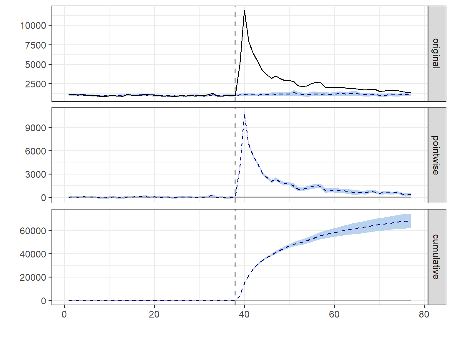

Summaries of the results

Code

summary(ci_m1)

Posterior inference {CausalImpact}

                         Average        Cumulative    
Actual                   2871           111962        
Prediction (s.d.)        1122 (84)      43776 (3262)  
95% CI                   [960, 1282]    [37451, 50002]
                                                      
Absolute effect (s.d.)   1748 (84)      68186 (3262)  
95% CI                   [1589, 1911]   [61960, 74511]
                                                      
Relative effect (s.d.)   157% (20%)     157% (20%)    
95% CI                   [124%, 199%]   [124%, 199%]  

Posterior tail-area probability p:   0.001
Posterior prob. of a causal effect:  99.8997%

For more details, type: summary(impact, "report")

Code

summary(ci_m1, "report")

Analysis report {CausalImpact}


During the post-intervention period, the response variable had an average value of approx. 2.87K. By contrast, in the absence of an intervention, we would have expected an average response of 1.12K. The 95% interval of this counterfactual prediction is [0.96K, 1.28K]. Subtracting this prediction from the observed response yields an estimate of the causal effect the intervention had on the response variable. This effect is 1.75K with a 95% interval of [1.59K, 1.91K]. For a discussion of the significance of this effect, see below.

Summing up the individual data points during the post-intervention period (which can only sometimes be meaningfully interpreted), the response variable had an overall value of 111.96K. By contrast, had the intervention not taken place, we would have expected a sum of 43.78K. The 95% interval of this prediction is [37.45K, 50.00K].

The above results are given in terms of absolute numbers. In relative terms, the response variable showed an increase of +157%. The 95% interval of this percentage is [+124%, +199%].

This means that the positive effect observed during the intervention period is statistically significant and unlikely to be due to random fluctuations. It should be noted, however, that the question of whether this increase also bears substantive significance can only be answered by comparing the absolute effect (1.75K) to the original goal of the underlying intervention.

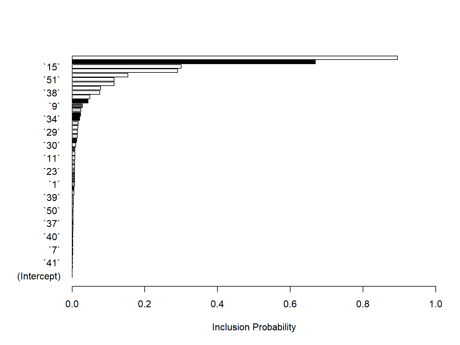
The probability of obtaining this effect by chance is very small (Bayesian one-sided tail-area probability p = 0.001). This means the causal effect can be considered statistically significant. 

Code

plot(ci_m1$model$bsts.model, "coefficients")

References

Arkhangelsky, Dmitry. 2023. Synthdid: Synthetic Difference-in-Difference Estimation. https://github.com/synth-inference/synthdid.

Arkhangelsky, Dmitry, Susan Athey, David A. Hirshberg, Guido W. Imbens, and Stefan Wager. 2021. “Synthetic Difference-in-Differences.” American Economic Review 111 (12): 4088–118. https://doi.org/10.1257/aer.20190159.

Bergé, Laurent. 2018. “Efficient Estimation of Maximum Likelihood Models with Multiple Fixed-Effects: The R Package FENmlm.” CREA Discussion Papers, no. 13.

Brodersen, Kay H., Fabian Gallusser, Jim Koehler, Nicolas Remy, and Steven L. Scott. 2014. “Inferring Causal Impact Using Bayesian Structural Time-Series Models.” Annals of Applied Statistics 9: 247–74. https://research.google/pubs/pub41854/.

Callaway, Brantly, and Pedro H. C. Sant’Anna. 2021a. “Did: Difference in Differences.” https://bcallaway11.github.io/did/.

———. 2021b. “Difference-in-Differences with Multiple Time Periods.” Journal of Econometrics, Themed Issue: Treatment Effect 1, 225 (2): 200–230. https://doi.org/10.1016/j.jeconom.2020.12.001.

R Core Team. 2022. R: A Language and Environment for Statistical Computing. Vienna, Austria: R Foundation for Statistical Computing. https://www.R-project.org/.

Rambachan, Ashesh, and Jonathan Roth. 2023. “A More Credible Approach to Parallel Trends.” The Review of Economic Studies, February, rdad018. https://doi.org/10.1093/restud/rdad018.

Sun, Liyang, and Sarah Abraham. 2020. “Estimating Dynamic Treatment Effects in Event Studies with Heterogeneous Treatment Effects.” Journal of Econometrics, December. https://doi.org/10.1016/j.jeconom.2020.09.006.

Xu, Yiqing, and Licheng Liu. 2021. Gsynth: Generalized Synthetic Control Method. https://yiqingxu.org/packages/gsynth/.